[49일차]이상탐지 실습

김준석·2024년 2월 1일

Today I Learned - 데브코스 데이터분석

데브코스_데이터분석-머신러닝 기초[10주차]

목록 보기

28/33

이상탐지 실습

캐글의 신용카드 거래 데이터를 가지고 실습을 진행해 보자

데이터 셋 설명

Credit Card Fraud Detection 데이터

Credit Card Fraud Detection

신용카드 거래에서의 사기 탐지를 위해 설계된 데이터셋
• 2013년 유럽 카드 소지자들의 거래 데이터를 포함
• 총 284,807건의 거래 데이터가 있고
• 그 중 492건(0.172%)의 사기 거래 데이터가 있음
```
그런데!! 데이터가 너무 커서 샘플링을 함.

- 전체 19,936건, 사기 34건 (0.171%) 데이터를 포함
```
변수로는 Time, Amount, V1~V28, Class
• Time : 첫 거래 후 각 거래 사이 경과 시간 (초)
• Amount : 거래 금액
• V1~V28 : PCA로 얻은 수치형 입력 변수
• Class : 정상 거래 (0)와 비정상 거래 (1)

문제정의

풀어야 하는 문제
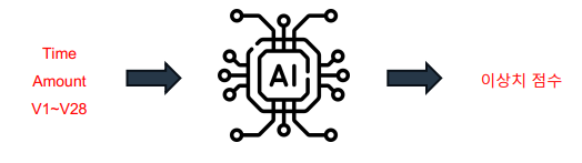
• 주어진 거래 관련 데이터를 바탕으로 이상 거래 데이터를 탐지

머신 러닝 모델의 입, 출력 정의
- 입력 : 거래 관련 데이터
  - Time
  - Amount
  - V1 ~ V28
- 출력 : 각 데이터 포인트 마다 할당된 이상치 점수 (종속 변수)
  - 후처리 필요

1. EDA

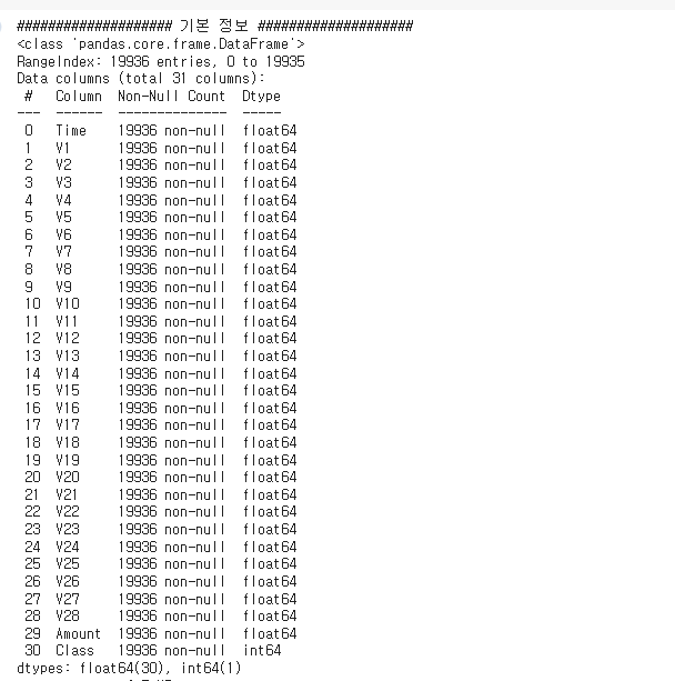
데이터는 독립변수 Time,V1~V28, Amount와 종속변수 Class가 있다.

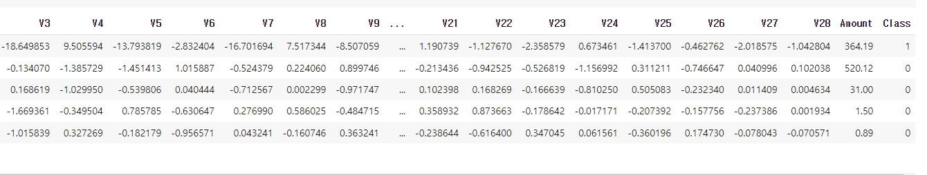
총 31개의 데이터로 결측치는 없는 모습!

기초 통계량은 패스!

범주형 데이터 (Class 컬럼) 분석

# 이상치 여부 시각화 (Class : 종속변수)
y_columns = ['Class']
y = credit[y_columns]

import matplotlib.pyplot as plt
plt.figure(figsize=(4, 4))

y.value_counts(normalize=True).plot(kind='bar', color=['b', 'r'])

plt.xticks(range(2), ['Nomal', 'Fraud'])
plt.title('Nomal VS Fraud')
plt.tight_layout()
plt.show()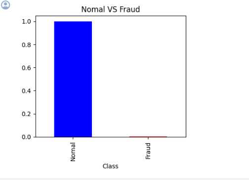

값이 Fraud가 너무 적다! 실제 갯수를 확인해 보자.

# 갯수 확인
num_Normal = (y==0).sum().values[0]
num_Fraud = (y==1).sum().values[0]
print(f'Number of Normal data : {num_Normal}')
print(f'Number of Fraud data : {num_Fraud}')

출력값:

Number of Normal data : 19902
Number of Fraud data : 34

확실히 작다. 이는 이상치로 분류할 수 있을 듯.

수치형 데이터 (시간, 거래 금액) 분석

# Time과 Amount 데이터

time_amount_columns = ['Time', 'Amount']
time_amount = credit[time_amount_columns]

# 분포 시각화
plt.figure(figsize=(6, 9))

np.random.seed(seed)
for idx, numeric in enumerate(time_amount_columns) :
    col = (np.random.random(), np.random.random(), np.random.random())

    plt.subplot(2, 1, idx+1)
    plt.hist(time_amount[numeric], bins=50, color=col, edgecolor='black')
    plt.title(numeric)
    plt.tight_layout()

plt.tight_layout()
plt.show()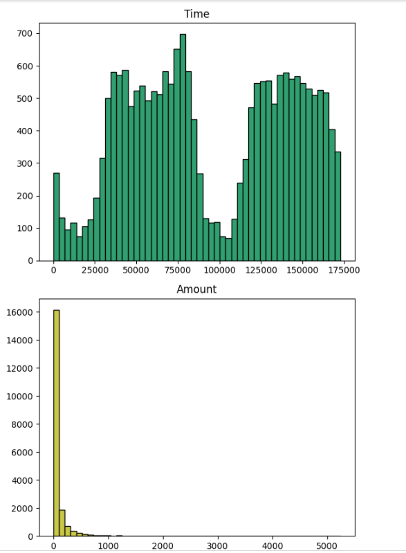

TIME!

Time의 경우 거래 시작 이후의 경과 시간을 나타내므로
기준 시간 정보가 있다면 주기성을 갖고 있을 수 있음

낮에 한 거래와 밤에 한 거래와 같이
그렇다면 주기 함수를 적용하는 것도 좋은 방법!

하지만 시간 그래프를 보면 175,000초(대략 2일) 정도까지 가지고 있다.
시작 지점이 정해져있지 않기 때문에 함수를 사용하는 것은 어렵다.

큰 outlier가 없어 보이므로 Min-Max Scaling 을 사용해서 시간대를 줄요보자.

AMOUNT!

Amount는 치우침이 있지만,
신용 카드 거래 금액으로 의미가 없는 데이터는 아님

근데 큰 값은 너무 작아서 그래프에서 보이지 않는다.

이처럼 극단적으로 치우쳐진 값을 처리하기 위해 Log 스케일링을 진행!

credit['Log_Amount'] = np.log(credit['Amount']+1)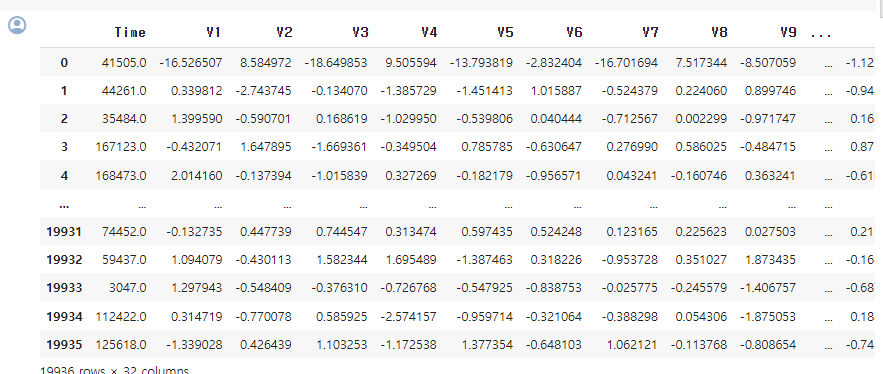

이를 시각화 하면!

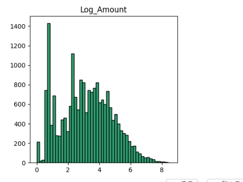
그럼 이렇게 예쁜 그래프가 나온다!

Log(0) 의 값을 피하기 위해 +1 값을 추가 해준다.
• Amount의 경우 1 정도의 크기가 큰 문제가 되지 않음
• 이 값이 영향을 미치는 데이터인지 확인 필요

2. 데이터 전처리 진행

Time : Min-Max Scailing
Amount : Log Amount 사용
V1 ~ V28 : 그대로 사용

Time 데이터 MinMaxScaler 처리

# Time 변수를 Min Max Scaling
from sklearn.preprocessing import MinMaxScaler
scaler = MinMaxScaler()

credit_time = scaler.fit_transform(credit[['Time']])
credit_time = pd.DataFrame(credit_time)
credit_time.columns = ['Time']
credit_time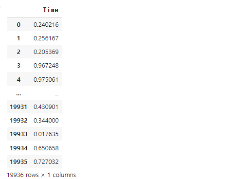

Amount 변수를 Log scale로 진행

# Amount 변수를 Log scale로

credit_log_amount= credit[log_amount_columns]
credit_log_amount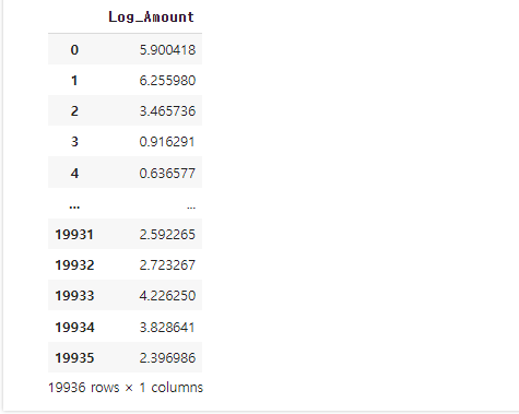

이를 데이터 프레임으로 합친다!

credit_combined = pd.concat([credit_time,
                             credit_log_amount,
                             Vs_data],
                            axis=1)
credit_combined

3. 모델 구축!

학습진행

n_estimators = 100
max_samples = 'auto'
# contamination = 'auto'
contamination = num_Fraud/(num_Normal+num_Fraud)

# Isolation Forest 생성 및 학습
from sklearn.ensemble import IsolationForest
IForest = IsolationForest(n_estimators=n_estimators,
                          max_samples=max_samples,
                          contamination=contamination,
                          random_state=seed)
IForest.fit(credit_combined)

contamination = num_Fraud/(num_Normal+num_Fraud) : 우리는 사기 갯수를 알기 때문에 임계치 비율을 완벽하게 기입함.

평가 진행

y_true = credit['Class']

y_pred = IForest.predict(credit_combined)
y_pred = np.where(y_pred == 1, 0, 1)

# 성능 평가
from sklearn.metrics import accuracy_score, precision_score, recall_score, f1_score

accuracy = accuracy_score(y_true, y_pred)
precision = precision_score(y_true, y_pred)
recall = recall_score(y_true, y_pred)
f1 = f1_score(y_true, y_pred)

print(f'정확도 Accuracy : {accuracy*100:.2f} %')
print(f'정밀도 Precision : {precision*100:.2f} %')
print(f'재현율 Recall : {recall*100:.2f} %')
print(f'F1 : {f1*100:.2f} %')

출력값:

정확도 Accuracy : 99.77 %
정밀도 Precision : 32.35 %
재현율 Recall : 32.35 %
F1 : 32.35 %

정확도 말고는 다 낮게 나왔다!!! 왜지!!

이를 confusion_matrix를 그려보면 알 수 있다.

from sklearn.metrics import confusion_matrix

result_cm = confusion_matrix(y_true, y_pred)

plt.figure(figsize=(6, 6))

plt.matshow(result_cm, fignum=1)
plt.xticks(range(2), [0, 1])
plt.yticks(range(2), [0, 1])
plt.ylabel('True label')
plt.xlabel('Predicted label')
plt.colorbar()

for (i, j), val in np.ndenumerate(result_cm):
    plt.text(j, i, f'{val}', ha='center', va='center', color='red')

plt.show()