참고한 커널을 거의 Copy한 정도이기 때문에 학습 등의 목적을 가지고 계신 분은 참고한 커널 Kaggle 공개 커널, 곽대훈님의 데이터 분석 어떻게 시작해야 하나요?로 이동해주세요.
이 글은 캐글 타이타닉으로 기초 쌓기 #3와 이어지는 내용입니다.
2. 탐색적 데이터 분석(EDA, Exploratory Data Analysis)
이제 어떤 feature가 Survived에 얼마나 영향을 미치는지 확인해보아야 합니다.
이를 위해서는 적절한 시각화가 필요합니다.
시각화 패키지는 matplotlib, seaborn, plotly 등이 있습니다.
본 커널에서는 matplotlib와 seaborn을 주로 사용할 것 입니다.
2.1 Pclass
가장 먼저 Pclass feature를 살펴봅시다.
Pclass는 서수(순서가 있는 수)형 데이터입니다. 즉, 카테고리 역할을 동시에 하는 데이터입니다.
pandas의 DataFrame에서는 SQL 쿼리의 groupby와 같은 groupby 메소드를 사용하면 쉽게 데이터를 묶어 볼 수 있습니다.
경우에 따라서는 pivot이라는 메소드를 사용해도 유용합니다.
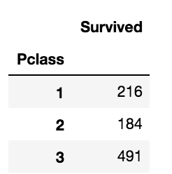
df_train[['Pclass', 'Survived']].groupby(['Pclass'], as_index=True).count()
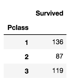
df_train[['Pclass', 'Survived']].groupby(['Pclass'], as_index=True).sum()
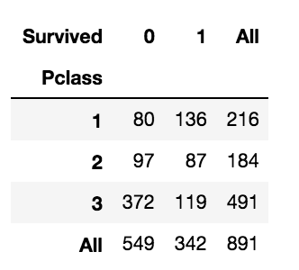
pd.crosstab(df_train['Pclass'], df_train['Survived'], margins=True)
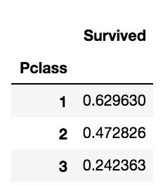
df_train[['Pclass', 'Survived']].groupby(['Pclass'], as_index=True).mean()
df_train[['Pclass', 'Survived']].groupby(['Pclass'], as_index=True).mean().plot.bar()Output[0]:
Output[1]:
Output[2]:
Output[3]:
Output[4]:
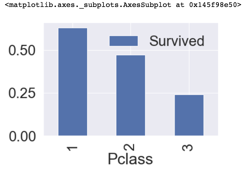
groupby 메소드를 이용하여 출력된 table을 보아도 Pclass feature가 Survived값에 큰 영향을 마친다고 확인 할 수 있습니다.
plot.bar 메소드를 통해 막대 그래프로 시각화하니 더 확실하게 알 수 있습니다.
2.2 Sex
이제 Sex feature를 확인해봅시다.
f, ax = plt.subplots(1, 2, figsize=(18, 8))

df_train[['Sex', 'Survived']].groupby(['Sex'], as_index=True).mean().plot.bar(ax=ax[0])
ax[0].set_title('Survived vs Sex')
sns.countplot('Sex', hue='Survived', data=df_train, ax=ax[1])
ax[1].set_title('Sex: Survived vs Dead')

plt.show()
Output:
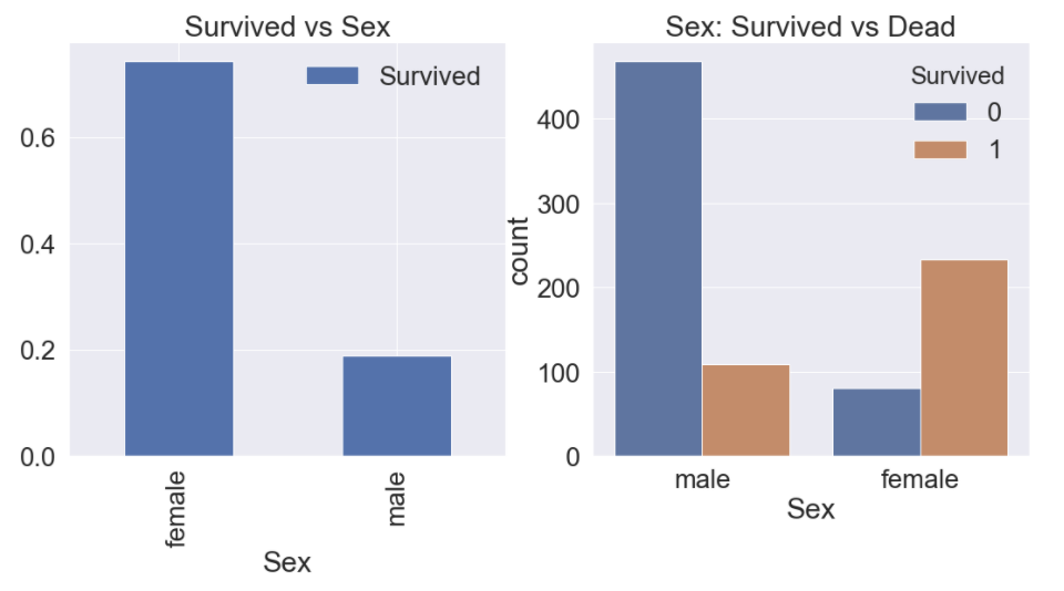
좌측의 막대 그래프를 보면 생존자 중 female인 passenger가 male인 passenger가 월등히 많음을 확인 할 수 있으며
각 Sex별 생존, 사망자 수를 비교해보아도 female인 passenger는 생존자가 더 많았으나 male인 passenger는 사망자가 더 많음을 확인 할 수 있었습니다.
이를 통해 Sex feature도 Survived에 큰 영향을 끼친다는 것을 알 수 있습니다.
2.3 Both Sex and Pclass
이번에는 Sex, Pclass 두 feature에 관해 생존이 어떻게 변화하는지 확인해봅시다.
sns.factorplot('Pclass', 'Survived', hue='Sex', data=df_train, size=6, aspect=1.5)Output:
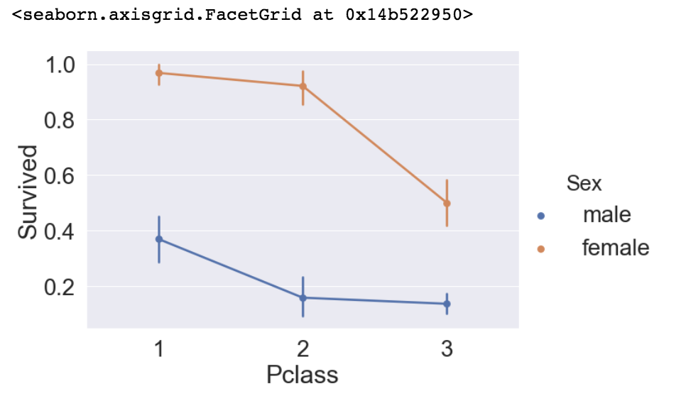
모든 Pclass, Sex에서 생존률이 male보다 female에 높음을 볼 수 있습니다.
2.4 Age
이번에는 Age feature에 대해 조사해봅시다.
fig, ax = plt.subplots(1, 1, figsize=(9, 5))

sns.kdeplot(df_train[df_train['Survived'] == 1]['Age'], ax=ax)
sns.kdeplot(df_train[df_train['Survived'] == 0]['Age'], ax=ax)
plt.legend(['Survived == 1', 'Survived == 0'])

plt.show()
Output:
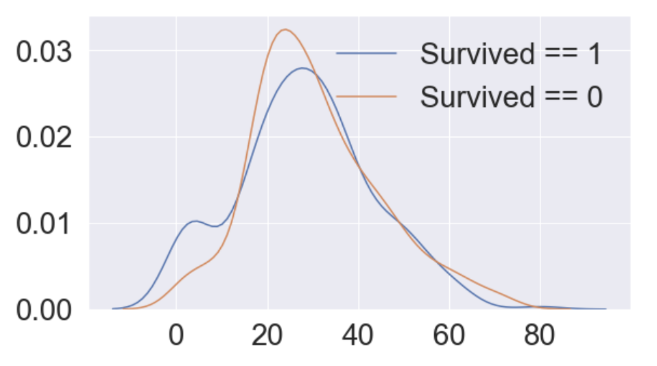
seaborn의 커널 밀도 분포를 곡선 그래프로 볼 수 있는 kdeplot 메소드를 이용하여 살펴본 결과, 전체적인 구간에서는 나이가 생존에 관계가 없어보이나 15세 미만 구간에서 특별하게 생존률이 높음을 확인할 수 있습니다.
plt.figure(figsize=(8, 6))
df_train['Age'][df_train['Pclass'] == 1].plot(kind='kde')
df_train['Age'][df_train['Pclass'] == 2].plot(kind='kde')
df_train['Age'][df_train['Pclass'] == 3].plot(kind='kde')

plt.xlabel('Age')
plt.title('Age Distribution within Pclasses')
plt.legend(['1st', '2nd', '3rd'])

plt.show()
Output:
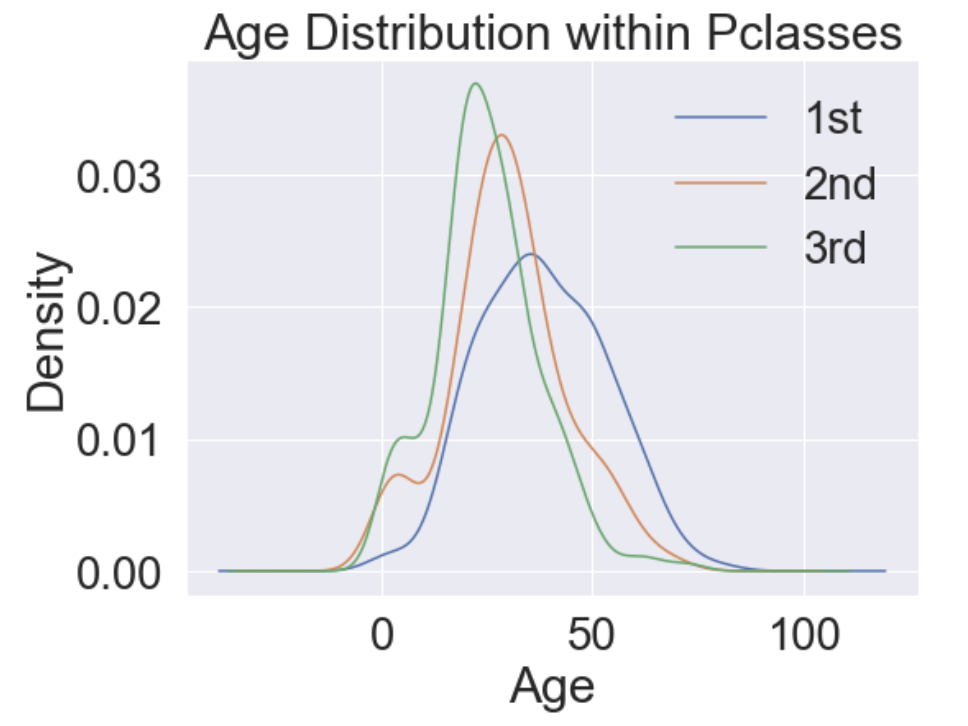
kdeplot을 통해 확인해보니 나이가 높을 수록 Pclass가 높습니다.
이젠 나이대가 높아짐에 따라 생존률 변화를 알기 위해 누적 확률을 활용한 시각화를 해봅시다.
- 누적 확률 개념 참고 : ratsgo님의 정규분포 누적분포함수와 중심극한정리
cumulate_survive_ratio = []
for i in range(1, 80):
    cumulate_survive_ratio.append(df_train[df_train['Age'] < i]['Survived'].sum() / len(df_train[df_train['Age'] < i]['Survived']))

plt.figure(figsize=(7, 7))
plt.plot(cumulate_survive_ratio)
plt.title('Survival rate change depending on range of Age feature', y=1.02)
plt.ylabel('Survival rate')
plt.xlabel('Range of Age(0 ~ x)')

plt.show()
Output:
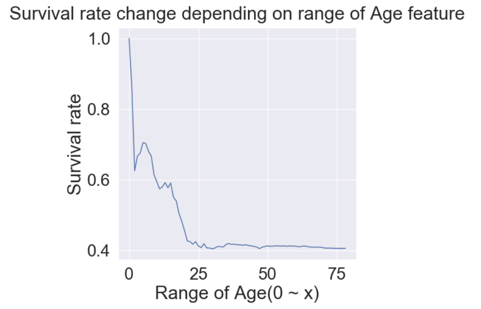
누적 확률을 통해 보았을 때 나이가 낮을 수록 생존률이 확실히 높은 것을 볼 수 있습니다.
나이도 중요한 feature입니다.
지금까지의 분석을 통해 얻은 정보를 정리하면
- 여자이거나
- 나이가 어리거나
- Pclass가 높을 수록(값이 낮을 수록)
생존률이 높음을 확인했습니다.
2.5 Embarked
Embarked feature는 passenger가 승선한 항구를 나타냅니다.
- C : Cherbourg
- Q : Queenstown
- S : Southampton
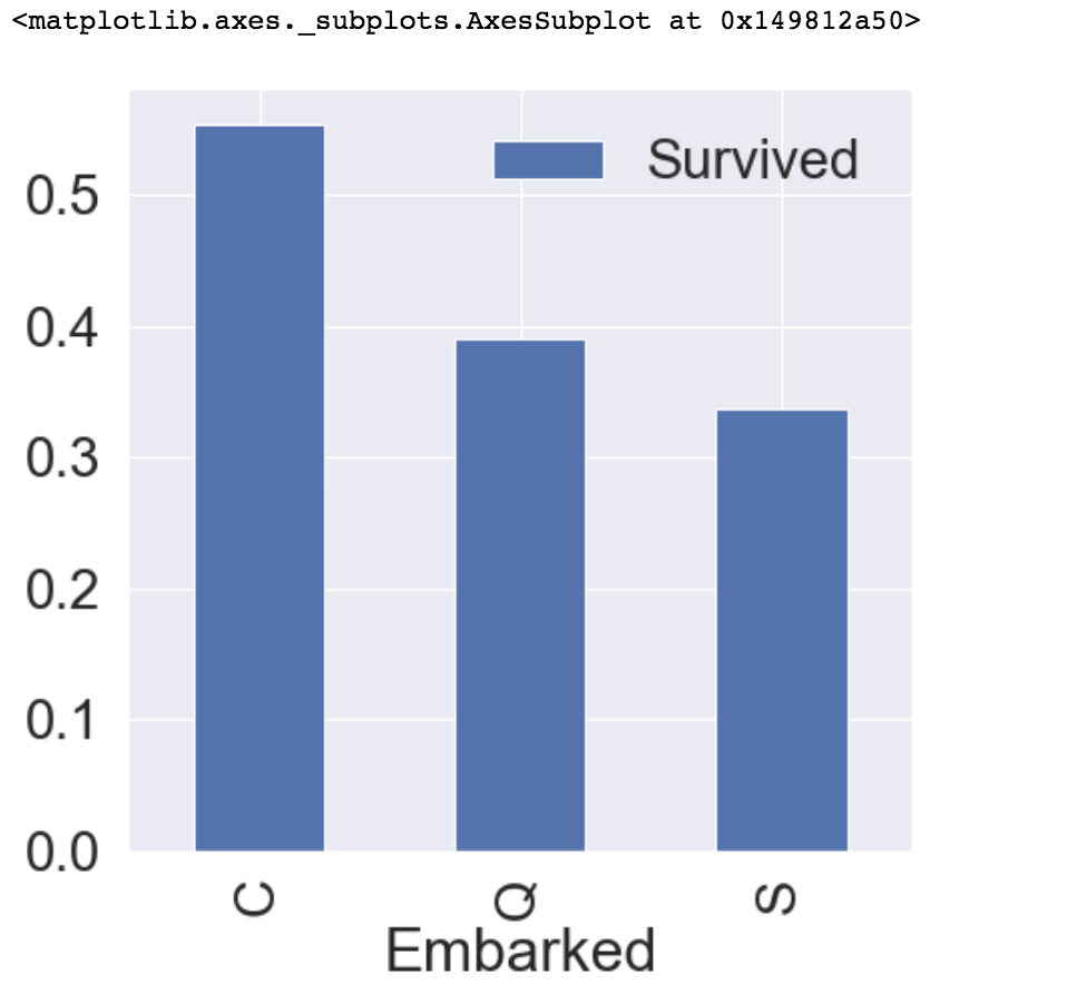
Embarked feature를 조사해봅시다.
df_train[['Embarked', 'Survived']].groupby(['Embarked'], as_index=True).mean().plot.bar(figsize=(7, 7))Output:
# 단순 Embarked feature에 따른 passenger 수를 막대 그래프로 시각화
fig, ax = plt.subplots(2, 2, figsize=(20, 15))
sns.countplot('Embarked', data=df_train, ax=ax[0, 0])
ax[0, 0].set_title('1. Number of passengers boarded')
# Sex feature를 카테고리로 막대 그래프 시각화
sns.countplot('Embarked', data=df_train, hue='Sex', ax=ax[0, 1])
ax[0, 1].set_title('2. Male-Female Split for Embarked')
# Embarked feature별 생존, 사망 수를 막대 그래프로 시각화
sns.countplot('Embarked', data=df_train, hue='Survived', ax=ax[1, 0])
ax[1, 0].set_title('3. Embarked vs Survived')
# 각 Embarked 별 Pclass 수를 막대 그래프로 시각화
sns.countplot('Embarked', data=df_train, hue='Pclass', ax=ax[1, 1])
ax[1, 1].set_title('4. Embarked vs Pclass')

plt.subplots_adjust(wspace=0.2, hspace=0.5) # figure가 겹치지 않게 간격 조절
plt.show()
Output:
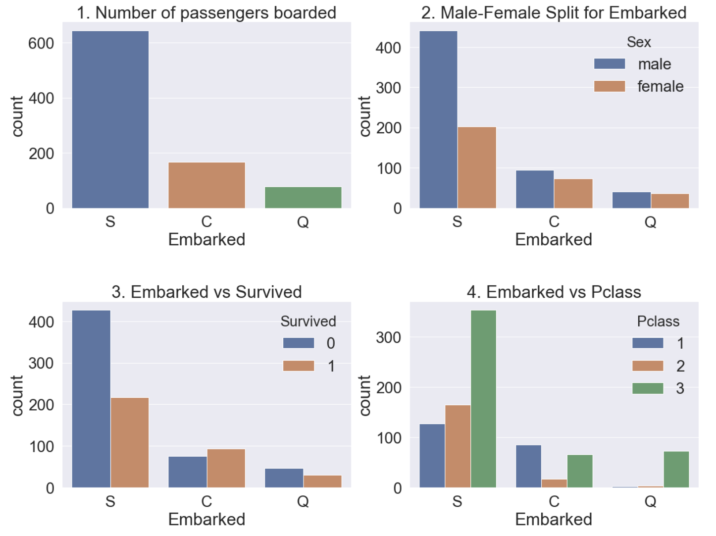
- Figure 1 - S(Southampton)에서 가장 많은 승객이 탑승했씁니다.
- Figure 2 - C(Cherbourg)와 Q(Queenstown)은 남녀 비율이 비슷하고 S는 남자가 더 많습니다.
- Figrue 3 - S의 경우 생존률이 특히 낮은 것을 볼 수 있습니다.
- Figure 4 - 이전 Pclass feature를 분석한 결과를 생각해보면 S에서 탑승한 Passenger가 Pclass가 낮은 승객 비율이 많기 때문에 생존확률이 낮게 나온 것으로 보입니다.
2.6 Family - SibSp + Parch
Sibsp(형제, 자매) feature와 Parch(부모, 자녀) feature를 합치면 같이 탑승한 가족의 수가 됩니다.
이 두 feature를 합쳐 Family라는 새로운 feature를 만들어서 생각해봅시다.
df_train['FamilySize'] = df_train['SibSp'] + df_train['Parch'] + 1 # 본인도 가족이기에 더해줍니다.
df_test['FamilySize'] = df_test['SibSp'] + df_test['Parch'] + 1

f, ax = plt.subplots(1, 3, figsize=(40, 10))
sns.countplot('FamilySize', data=df_train, ax=ax[0])
ax[0].set_title('1. Number of passenger boarded', y=1.02)
sns.countplot('FamilySize', data=df_train, hue='Survived', ax=ax[1])
ax[1].set_title('2. Survived countplot depending on FamilySize', y=1.02)
df_train[['FamilySize', 'Survived']].groupby(['FamilySize'], as_index=True).mean().sort_values(by='Survived', ascending=False).plot.bar(ax=ax[2])
ax[2].set_title('3. Survived rate depending on FamilySize', y=1.02)

plt.subplots_adjust(wspace=0.2, hspace=0.5)
plt.show()
Output:
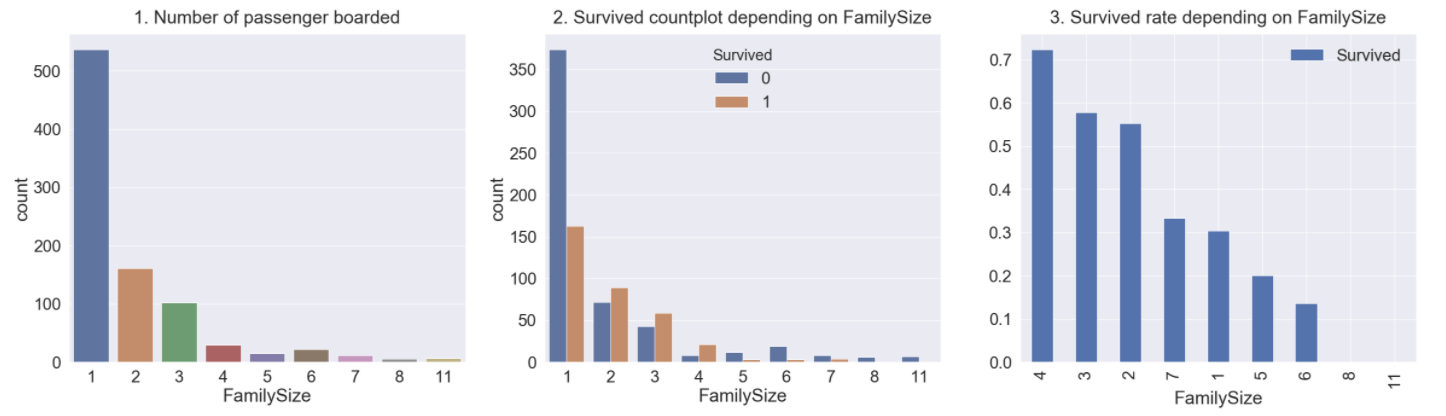
- Figure 1 - 혼자서 탑승한 passenger가 가장 많고 그 다음으론 순서대로 2, 3, 4명입니다.
- Figure 2, 3 - 2, 3, 4명 단위로 탑승한 가족의 경우 생존 비율이 더 높았고 그 외에는 사망률이 더 높습니다. 또한, 가족수가 너무 작거나 크면 생존률이 떨어지는 것을 확인할 수 있습니다. 2~4명의 경우 생존률이 가장 높습니다.
2.7 Fare
Fare feature는 탑승 요금입니다.
해당 feature는 연속 데이터이므로 histogram을 통해 시각화해봅시다.
fig, ax = plt.subplots(1, 1, figsize=(10, 10))
g = sns.distplot(df_train['Fare'], color='b', label='Skewness: {:.2f}'.format(df_train['Fare'].skew()), ax=ax)
g = g.legend(loc='best')

plt.show()
Output:
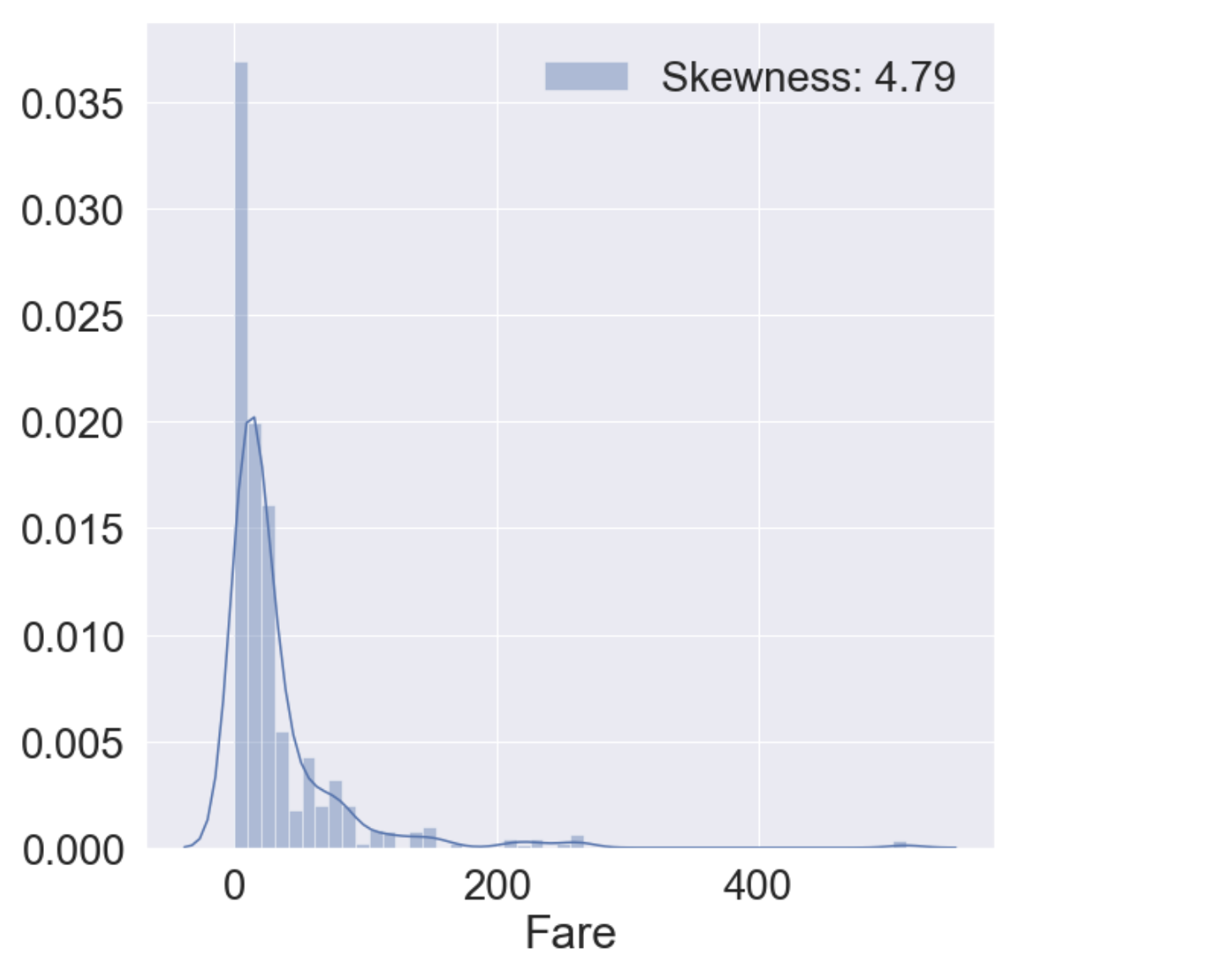
참고 커널에서는 Fare 데이터에 log를 취해 비대칭성을 최소화한다.
해당 커널 작성자는 이후 Feature engineering을 진행할 때 필요한 부분인데 미리 작업한 것이라고 했기에 일단 따라서 작성하고 이후 해당 과정을 진행할 때 이해하보도록 하겠습니다.
df_test.loc[df_test.Fare.isnull(), 'Fare'] = df_test['Fare'].mean()
# test.csv의 데이터에서 이상하게 1개의 row가 Fare 값이 null이기 때문에 평균값으로 처리해줍니다.
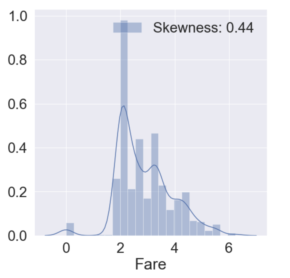
df_train['Fare'] = df_train['Fare'].map(lambda i: np.log(i) if i > 0 else 0)
df_test['Fare'] = df_test['Fare'].map(lambda i: np.log(i) if i > 0 else 0)
fig, ax = plt.subplots(1, 1, figsize=(8, 8))
g = sns.distplot(df_train['Fare'], label='Skewness: {:.2f}'.format(df_train['Fare'].skew()))
g = g.legend(loc='best')Output:
2.9 Ticket
이 feature는 티켓 번호입니다. 또한 NaN이 없는 String Type의 데이터인데 이 데이터를 가공을 해야만 실제 모델에 사용할 수 있습니다.
규칙성이 없어보이고 매우 다양합니다. 이를 모델에 사용하기 위해서는 아이디어가 필요합니다.
참고한 커널의 작성자는 이 feature를 사용하지 않아 타이타닉 문제를 풀이하고 이후 학습을 끌어올리기 위해 해보아야겠습니다.