분류

MNIST

분류 데이터셋으로 가장 유명한 MNIST 데이터셋을 사용하였습니다.

import numpy as np
from sklearn.datasets import fetch_openml
mnist = fetch_openml('mnist_784',version=1)
X, y = mnist["data"], mnist["target"]

위의 코드를 이용하여 사용할 수 있습니다.

이진 분류

문제를 예 / 아니오 로만 구별하는 분류기가 이진 분류기입니다.

SGD(확률적 경사 하강법)Classifier를 사용해보았습니다.

• SGD분류기는 무작위성을 가지고 있어 Stochastic이 붙었습니다.

성능 측정

교차검증

가장 먼저 교차검증이 있습니다.
교차검증은 아래와 같은 kFold를 이용하거나 cross_val_socre()를 이용해서 할 수도 있습니다.

• 5인지 아닌지 분류하는 이진 분류기

from sklearn.model_selection import StratifiedKFold
from sklearn.base import clone

skfolds = StratifiedKFold(n_splits=3, random_state=42)

for train_index, test_index in skfolds.split(X_train, y_train_5):
  clone_clf = clone(sgd_clf)
  X_train_folds = X_train[train_index]
  y_train_folds = y_train_5[train_index]
  X_test_fold = X_train[test_index]
  y_test_fold = y_train_5[test_index]

  clone_clf.fit(X_train_folds, y_train_folds)
  y_pred = clone_clf.predict(X_test_fold)
  n_correct = sum(y_pred == y_test_fold)
  print(n_correct / len(y_pred))

from sklearn.model_selection import cross_val_score
cross_val_score(sgd_clf, X_train,y_train_5, cv=3, scoring="accuracy")

이때 정확도를 성능기준으로 사용하였는데,
이처럼 불균형한 데이터셋일 때는 성능 측정 지표로 좋지 않습니다.

만약 무조건 5가 아니라는 결과만 내는 분류기의 성능을 정확도를 기준으로 측정한다면
5가 데이터셋에 적게 들어있는 만큼 높은 성능이 나올 것이기 때문입니다.

이로 인해 오차 행렬에 대해 알아보아야 합니다.

오차 행렬

confusion matrix를 보여주기 위해 cross_val_predict()를 사용하여
k겹 교차 검증을 수행하지만 평가 점수를 반환하지 않고 각 테스트 폴드에서 얻은 예측을 반환하기 하도록 합니다.

from sklearn.model_selection import cross_val_predict
y_train_pred = cross_val_predict(sgd_clf, X_train, y_train_5, cv=3)

from sklearn.metrics import confusion_matrix
confusion_matrix(y_train_5, y_train_pred)

왼쪽부터 차례대로

true Negative, false positive

false Negative, true Positive 입니다.

정밀도 : TP / (TP + FP)

• 정밀도는 분류기가 예측한 Positive 중에서 진짜 positive의 비율을 보여줍니다.

재현율 : TP / (TP + FN)

• 재현율은 진짜 Positive 중에서 분류기가 얼만큼 Positive로 예측을 하였는지의 비율을 보여줍니다.
• 민감도 또는 TPR(진짜 양성 비율)이라고도 합니다.

- TP: 진짜 Positive의 수 - FP: 거짓인데 Positive로 나온 수

정밀도와 재현율은 트레이드오프로 둘 중 하나가 올라가면 다른 하나는 내려가기 쉽습니다.
이를 한번에 보기 편하도록 F1 score를 이용할 수도 있습니다.
F1 score는 정밀도와 재현율의 조화 평균을 말합니다.

 from sklearn.metrics import f1_score
 f1_score(y_train_5, y_train_pred)

정밀도와 재현율 트레이드오프

먼저 precision_recall_curve로 모든 임계값에 대해 정밀도와 재현율을 계산할 수 있습니다.

from sklearn.metrics import precision_recall_curve
precisions, recalls, thresholds = precision_recall_curve(y_train_5, y_scores)

def plot_precision_recall_vs_threshold(precisions, recalls, thresholds):
 plt.plot(thresholds, precisions[:-1],"b--",label="precision")
 plt.plot(thresholds, recalls[:-1],"g-",label="recall")
 plt.legend()
 plt.xlabel("threshold")
 plt.show()
plot_precision_recall_vs_threshold(precisions, recalls, thresholds)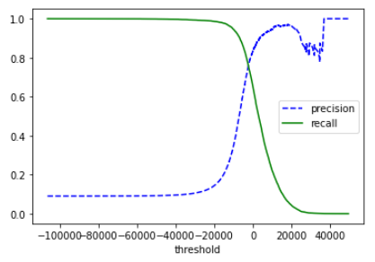

• 정밀도가 급격하게 줄어드는 하강점 직전이 주로 threshold로 좋습니다.

ROC 곡선

• FPR에 대한 TPR의 곡선
• 재현율에 대한 1-특이도 그래프

FPR : 양성으로 잘못 분류된 음성 샘플의 비율, 1-TNR
TNR : 특이도
TPR : 재현율

from sklearn.metrics import roc_curve
fpr, tpr, thresholds = roc_curve(y_train_5, y_scores)

def plot_roc_curve(fpr, tpr, label=None):
  plt.plot(fpr, tpr, linewidth=2, label=label)
  plt.plot([0,1],[0,1],'k--')
  plt.xlabel('FPR')
  plt.ylabel('TPR')
  
plot_roc_curve(fpr,tpr)
plt.show()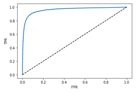

• AUC(곡선 아래 면적)가 1이면 완벽한 분류기이며, 0.5이면 완전한 랜덤 분류기 입니다.

from sklearn.metrics import roc_auc_score
roc_auc_score(y_train_5, y_scores)

다중 분류

다중분류에는 2가지 전략이 있다.
OvR, OvO

OvR( One versus the rest ) 전략

• 이진 분류기 n개를 이용하여 클래스가 n개인 이미지 분류 시스템 만드는 것.
• 이때 각 분류기의 결정 점수 중에서 가장 높은 것을 클래스로 선택

OvO( One versus one ) 전략

• 0과 1 구별, 0과 2 구별, 1과 2 구별 등 각 숫자의 조합마다 이진 분류기 훈련시키는 것
• N개의 클래스 -> N * (N-1) / 2개의 분류기 필요

• 서포트 벡터 머신은 이진분류기이기 때문에 사이킷런 내부에서 OvO전략을 사용해서
  10개의 분류기를 훈련시키고 각각의 결정점수를 얻어 가장 높은 클래스를 선택했을 것

from sklearn.svm import SVC
svm_clf = SVC()
svm_clf.fit(X_train,y_train)
svm_clf.predict([some_digit])

some_digit_scores = svm_clf.decision_function([some_digit])

print(np.argmax(some_digit_scores))
print(svm_clf.classes_)
print(svm_clf.classes_[5])

OvO, OvR를 강제로 사용하게 할 수도 있다.

from sklearn.multiclass import OneVsRestClassifier
ovr_clf = OneVsRestClassifier(SVC())
ovr_clf.fit(X_train, y_train)
ovr_clf.predict([some_digit])

다중 레이블 분류

• 아래의 KNN분류기로 7보다 높은 수인지 아닌지, 홀수 인지 아닌지 2개의 레이블을 가지고 분류할 수 있다.

from sklearn.neighbors import KNeighborsClassifier

y_train_large = (y_train >= 7)
y_train_odd = (y_train %2 == 1)
y_multilabel = np.c_[y_train_large, y_train_odd]

knn_clf = KNeighborsClassifier()
knn_clf.fit(X_train, y_multilabel)

knn_clf.predict([some_digit])

y_train_knn_pred = cross_val_predict(knn_clf, X_train, y_multilabel, cv=3)
f1_score(y_multilabel, y_train_knn_pred, average="macro")

• 모든 레이블의 가중치가 같지 않다면(데이터 비율이 다르다) 레이블에 클래스의 지지도(타깃 레이블에 속한 샘플 수)를 가중치로 둘 수도 있다.

  average="weighted"