8. Approximation Algorithm (1)

8.0 Approximation Algorithm

8.0.1 Strategy of Problem Solving

If a target problem is easy

• Find an algorithm working in polynomial time

Otherwise

• Do not spend so much time on developing a polynomial time algorithm or reduce its time complexity
• Give up accuracy or budget
  • Invest money for buying a supercomputer
    • 현실적으로 불가능
  • Build an algorithm working in polynomial time by giving up accuracy

문제가 어려울 때, 다항식 시간 알고리즘을 개발하거나 시간 복잡도를 낮추는 데 시간을 쏟을 필요 없다. 이때는 정확도나 비용 중 하나를 포기하고 Greedy 같은 방법으로 다항식 시간 내에 실행 가능한 근사 알고리즘을 설계한다.

근사 알고리즘은 최적해를 찾는 대신 근사해를 찾으면서 다항식 시간의 복잡도를 가진다.

Complexity of problem

• Deterministrically polynomial time $\rightarrow$ easy
• Otherwise $\rightarrow$ complex (i.e., NP-hard, NP-completeness)
• NP-completeness theory

Trade-Off between Time and Accuracy

• Spend more time (high time complexity) $\rightarrow$ higher accuracy
• Spend less time $\rightarrow$ less accurate
  • Some algorithm is not working for this purpose
• The second idea: appoximation algorithm

How to reduce the running time of algorithm?

• Prune search space by hypothesis
• Search until you find a relatively good solution
• Many probabilistic techniques
• Leads to AI algorithms (search algorithms)

Search space를 Prunning하면 정답이 존재하는 공간을 날릴 수도 있기 때문에 실제 정답과의 차이가 존재할 수 있다.

• In the other view
  • Time (not polynomial)
  • Reduce problem size(we solve only for a subset of input cases)
  • Find an approximation to the optimal solution

search space와 다르게 문제의 조건이나 입력 범위를 줄여서 일부만 해결한다. 문제를 특정 조건에 한정해 적용하거나, 제한된 범위 내에서만 풀도록 설계한다.

8.0.2 Approximation Ratio

Goal

• Practically runnable (working in polynomial time)
• Find a good solution

다항식 시간 내 동작하는 좋은 해를 찾자.

How good solution we need to find?

• Of course, finding an optimal solution is the best
• but highly likely, it is proven impossible to solve in polynomial time
  $\rightarrow$ Maximize the quality of solution as much as possible

실제 정답의 값을 Lower bound로 삼고 근사 알고리즘으로 구한 해의 값을 upper bound를 잡아 두 값의 비율을 계산하면 근사 비율이 된다. 근사 비율은 알고리즘이 최적해에 얼마나 가까운지, 즉 품질이 어느정도인지를 나타낸다.

구할 수 없는 최적해를 대신할 수 있는 "간접 최적해"를 찾고, 이를 최적해로 삼아서 근사 비율 계산

Approximation Ratio

• How to evaluate "goodness" (quality) of generated solutions?

Correct solution is unknown

• Just maximize the quality
• Benchmark test
  • for a few input cases whose corresponding solutions are already known
• Analyze upper bound of errors $\rightarrow$ Approximation ratio analysis
  • Using a virtual solution
  • Relation to a correct solution should be known
  • Quality is calculatable

---

8.1 Traveling Salesman Problem

Goal

• Find the path to minimize its weight sum

Conditions

• A path is given
• A traveler starts from a node
  • Visits all nodes once
  • Comes back to the starting node

TSP는 해밀턴으로부터 reduction 할 수 있다. 해밀턴은 주어진 그래프에서 모든 정점을 정확히 한 번씩 방문하는 순환이 존재하는지를 묻는 결정 문제이고, TSP는 그러한 순환들 중 최소 가중치 합을 갖는 경로를 찾는 최적화 문제이다.

해밀턴을 TSP로 변환할 때는 원래 그래프의 간선에 가중치를 1로 부여하고, 존재하지 않는(TSP는 완전 그래프이므로) 간선은 가중치를 $\infin$로 둔다.

Variations of TSP

• Many different conditions
• Conditions used in this lecture
  • Symmetry
    • A $\rightarrow$ B = B $\rightarrow$ A
  • Triangle inquality
    • A $\rightarrow$ B < A $\rightarrow$ C $\rightarrow$ B
  • Positive or zero weight
  • (Geometric distance: weight)

8.1.1 Design of an appoximation algorithm

• TSP: NP-complete $\rightarrow$ too complex $\rightarrow$ decision to approximate the solution
• How to?
  • Find a similar problem
    • Minimun Spanning Tree: all node visiting and weight sum minimization
  • Get a polynomial time algorithm
    • Kruskal, Prim
  • Convert the algorithms to satisfy additional conditions (not path, cycle)
• In this case,
  • Applying MST $\rightarrow$ get the results $\rightarrow$ convert it to a candidate solution for TSP

MST 알고리즘의 해를 바로 TSP 해로 쓸 수는 없고, 사이클을 어떻게 만들지 추가 변환 과정이 필요하다.

8.1.2 Process of Conversion

Process of Conversion

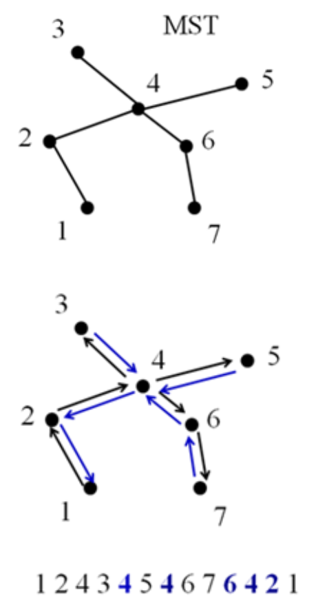
1. Find an MST
   • 완전 그래프에서 MST 찾기
2. Select one starting node
3. Allow repeated visiting node (node1 or given node)
   • DFS, 해가 유일하진 않음
4. Draw a cycle
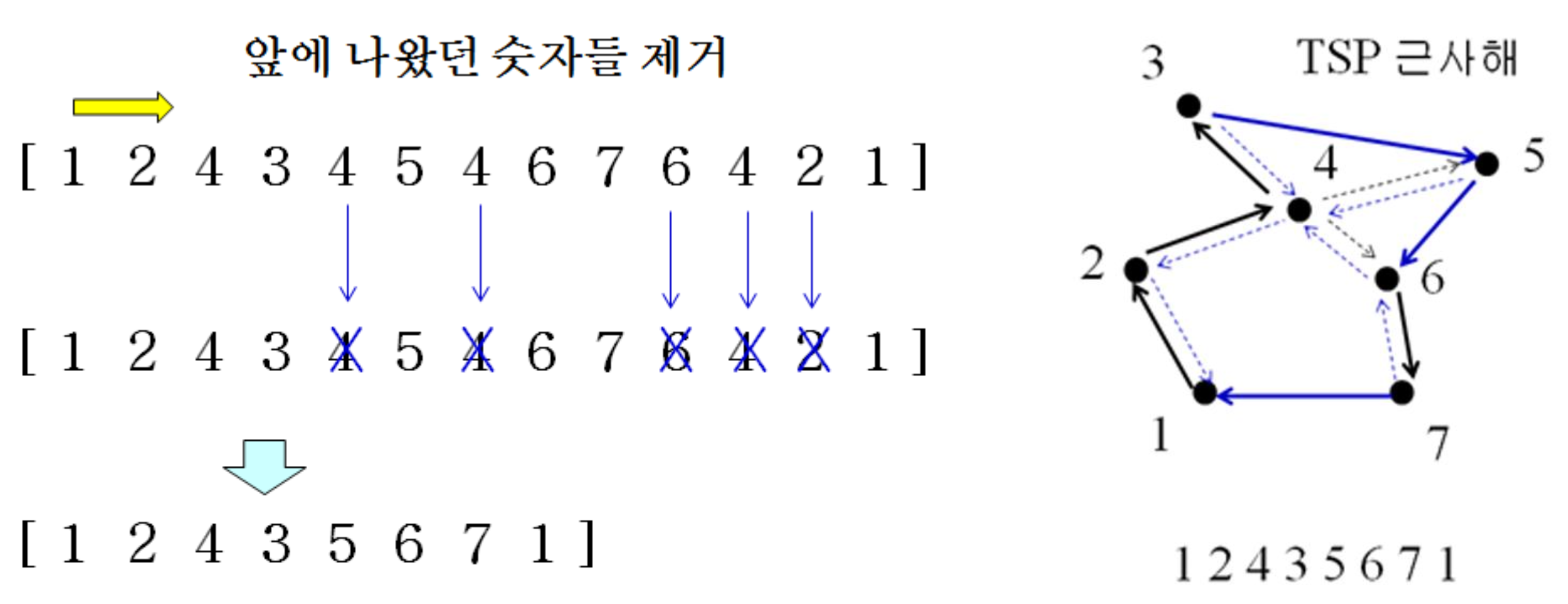
   • [1 2 4 3 4 5 4 6 7 6 4 2 1]
5. Remove duplicated nodes in the cycle
   • due to the TSP condition

cycle에서 1을 제외한 중복 도시를 모두 제거하면 된다.

DFS(깊이 우선 탐색)

• 한 방향으로 끝까지 가보고 막히면 되돌아와서 다른 길을 탐색하는 방법
• 모든 노드를 체계적으로 방문
• 각 간선을 정확히 2번 지남; 내려갈 때 1번, 올라갈 때 1번

How to remove the duplicated nodes?

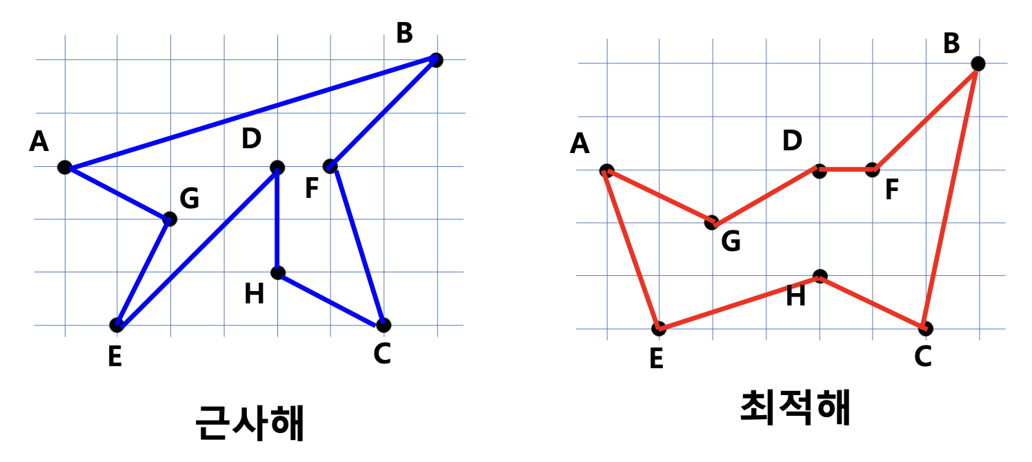
• Triangle inequality holds when we apply the deletion $\rightarrow$ decrease by each deletion

삼각 부등식 덕분에 중간 노드를 건너뛰어도 거리가 늘어나지 않는다.

8.1.3 TSP()

• Input: a weighted graph
• Output: a simple path starting from and ending to a randomly selected node

1. Find a MST (by Kruskal or Prim) - $O(nlogn)$ or $O(n^2)$
2. Convert a MST to a TSP path - $O(n)$
3. Remove repeatedly visited nodes in the path - $O(n)$
4. Return the simplest path

Total Complexity

• $O(nlogn)$ or $O(n^2)$

8.1.4 Approximation Ratio

• Esimation correct ratio is the best, but usually impossible
• Find an upper bound of error
  • Still hepful to make a decision of using your algorithm
• If correct solutions are unknown?
  • Use a virtual but clearly better than correct solution

Approximation Ratio = (근사 알고리즘의 해) / 최적해

TSP의 최적해를 실질적으로 알 수 없으므로 간접적인 최적해인 MST 간선의 가중치 합을 최적해의 값으로 활용한다.

Approximation ratio of MST convesion algorithm for TSP

• A virtual solution for TSP: MST
  • Weight sum of MST: $M$ (assumption)
  • Weight sum of the best solution for TSP $C$
  • $C>M$

왜 $C > M$임을 확신할까?
M은 edge 수가 tree 구조이므로 n - 1이고, C는 cycle이므로 n개이다.

• A lower bound for the correction solution
  • TSP is a cycle: N edges
  • MST is a path: N - 1 edges
  • Remove one edge from the best TSP solution
    • a spanning tree > minimum spanning tree
• A upper bound for the approximated solution
  • Weight sum of the approximation: M" (cycle O)
  • M" < 2M
  • We use each edge twice to build a cycle from the MST $\rightarrow$ 2M
  • Any reduction decreases the weight sum from 2M

Approximation Ratio

• A lowerbound of correct solution M
  • TSP의 올바른(최적) 해의 비용은 M 이상
• An upperbound of approximation 2M
  • MST 변환 방식으로 얻은 근사 해의 비용은 최대 2M, 최적해보다 2배 이하
• Approximation ratio = cost of appoximation / cost of correct solution = M"/M'

최악의 경우 candidate 값이 2배까지 늘어난다.

---

8.2 Vertex Covering

Goal

• Find a node set to cover all edges with minimal cadinality

Conditions

• A graph is given
• An edge is "covered" if its one node is in the set

E.g.,

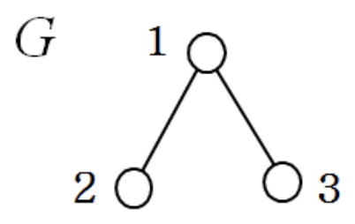
• (Vertex) Sets to cover all edges: {1, 2, 3}, {1, 2}, {1, 3}, {2, 3}, {1}
• Incorrect sets: {2}, {3} (not all edges are covered)
• Minimal cardinality: {1} $\rightarrow$ corrrect solution

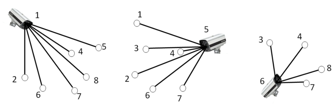
E.g.,

• Practical Application
• Edeges: aisles to watch through CCTV
• Nodes: candidates positions of CCTV
• How to minimize the number of CCTV to cover all aisles
  • {1, 5, 6}

8.2.1 Approximation Ratio of Greedy Algorithm for Vertex Covering

Greedy Vertex Cover는 왜 항상 최적해를 못 찾을 수 있는지 보여주는 예시이다.

• Greedy Algorithm for Vertex Covering
• Select the most frequenctly used node in all edges
• Skip nodes adjacent nodes to the selected node
• Repeat the process until all edges are covered

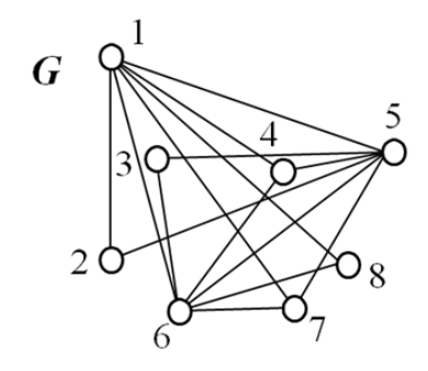
• A failed graph to find the best solution through a greedy algorithm

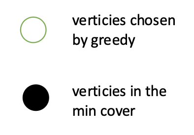
검은 정점들이 실제로는 최소 vertex cover를 이루는 정점들이지만, greedy의 선택은 연두색 원이 된다.

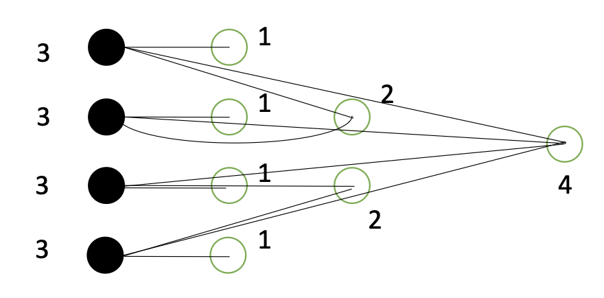
8.2.2 Another Greedy Algorithm

• Select edges instead of verticies
• One selected edge $\rightarrow$ two selected verticies
• E: selected edges
• V: verticies of e in E
• Select a disjoint edge (a set of verticies) with selected V
• Repeat until there is no disjoint edge

정점 대신에 간선을 greedy하게 뽑고, 그 간선의 두 끝점을 모두 cover에 넣는다.

E.g.,

• Select an edge first intially from G
• Edges sharing a node with the selected edge are coverd
• They can not be selected again
• A set of such edges (no node sharing) is a "matching"

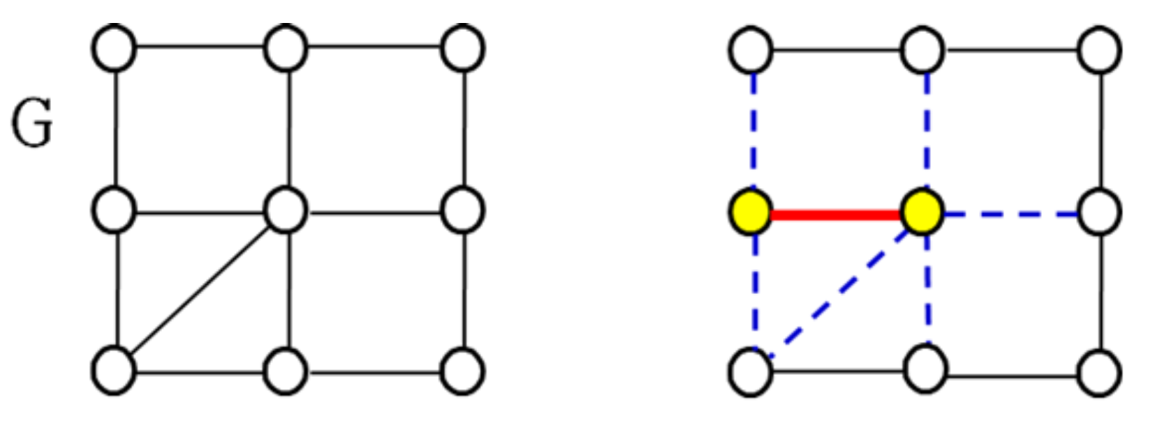
노란 정점 두 개를 넣으면서 두 정점과 연결된 모든 간선(파란 점선)이 이미 cover된 간선이 된다.

E.g.,

• If there is no more edge to add, the edge is a "maximal matching"
• Provide an approximation to the set covering problem

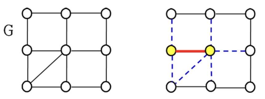
파란 점선 간선들은 '이제 못 고르는 간선들'이 되어 간선을 더 이상 추가할 수 없을 때까지 선택하면 얻어진 간선 집합이 maximal matching M이다.

8.2.3 Approx_Matching_VC

• Input: G = (V, E)
• Output: a set of nodes to cover all edges

1. find the maximal matching M
2. return the nodes used for M

• Matching: 각 간선의 양쪽 끝점들이 중복되지 않는 간선의 집합
• Maximal matching: 이미 선택된 간선에 기반을 두고 새로운 간선을 추가하려 해도 더 이상 추가할 수 없는 matching

Maximal matching을 이용해 정점 커버를 해결하자. 간선의 양 끝점이 이미 커버된 간선의 끝점이 아닐 때에만 선택한다.

Maximal Matching

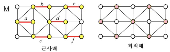
• Maximal matching: {a, b, c, d, e, f} edge set
• Node set M: {nodes of a, b, c, d, e, f}
• | M | = 12
  • 간선 1개당 정점 2개이므로 6 $\times$ 2 = 12
• The cardinality of the correct solution = 7

8.2.4 Time Compleity

Time Complexity of Approx_Matching_VC

• To select one edge, whether there is a shared node in V: $O(n)$
• | E | = m
• Repeat selection by m times in the worst case: $O(nm)$
  • 간선마다 검사 비용이 $O(n)$이고, 최악에는 $m$번 반복할 수 있으므로 최대 $O(nm)$

Can we achieve $O(mlogn)$?

• Union-Find algorithm
• Use heap tree
• V: a heap tree

1. Check a node is in V: $O(log n)$
   • update who is the root of V
2. Insertion of who nodes to V: $O(2 log n) ~ O(log n)$
3. $O(log n)$ to select one edge

간선 하나 처리 시간 $O(n)$에서 자료구조를 바꿔서 이 연산을 $O(log n)$으로 줄인다.

$m \times O(log n)$ $\rightarrow$ $O(m log n)$

8.2.5 Approximation Ratio

S: Maximal matching - 알고리즘이 선택한 간선들의 집합

• | S | = M: the number of edges(간선) in the maximal matching S
• | T | = M': the number of verticies(정점) of true optimal T
• M"=2M: the number of verticies in S (근사 알고리즘으로 찾은 정점의 개수)

Axiom 1

• All verticies of edges in S are unique (by definition)

Axiom 2

• All edges should be covered by T (by definition)

T가 최대이므로 더 큰 매칭이 없어 모든 간선이 T 정점들에 인접합니다.

Lemma 1

• | T | >= | S | (M' > M)
  • S is a subset of E (by definition)
  • T should cover S (by axiom 2)
  • If a vertex $v$ in T covers $e$ in S, $v$ is never used in another $e$ in S (by axiom 1)
  • To cover all $e$ in S, we need at least $v$ as | S |

Approximation Ratio

• M" = 2| S | = 2M (by definition of maximal matching)
• M" = 2M < 2M' (M' > M by lemma 1)
• M" / M' < 2 (Approximation ratio)

최악도 2배보다는 작다.

---

8.3 Bin Packing

Goal

• Find the minimum number of bins to put the given all objects

Conditions

• $n$ objects are given
• Each bin has volume limit $C$
• Objects in a bin can not have larger volume than $C$
• The order of objects is fixed

E.g.,

• $C$ = 10
• 3 bins spent 6, 5, and 8

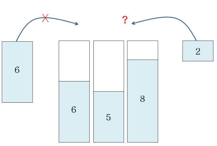
• Volume of next object to put is 6
  • Use a new bin
• Volume of next object to put is 2
  • Which bin you will use?
    $\rightarrow$ Greedy

8.3.1 Greedy Algorithm for Bin Packing

1. First fit

• Use the first avaliable bin to put the new object

2. Next fit

• Use the previosly used bin to put the new object

3. Best fit

• Use the avaliable bin to have smallest remaining space after putting the object

4. Worst fit

• Use the avaliable bin to have largest remaining space after putting the object

Worst fit을 왜 사용할까?
Bin을 동적으로 생성할 때마다 발생하는 초기화나 할당 overhead가 크기 때문이다. 처리 초반에 여러 bin을 미리 생성한 후, worst fit으로 가장 여유 공간이 큰 bin에 배치함으로써 빈 생성 비용을 최소화하고 전체 성능을 개선할 수 있다.

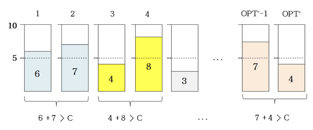
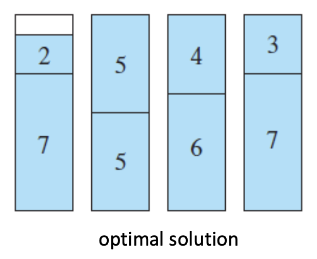
E.g., C = 10, object volumes = [7, 5, 6, 4, 2, 3, 7, 5]

Optimal Solution

• More Strategy
• Last fit, First fit decrease, Best fie decrease

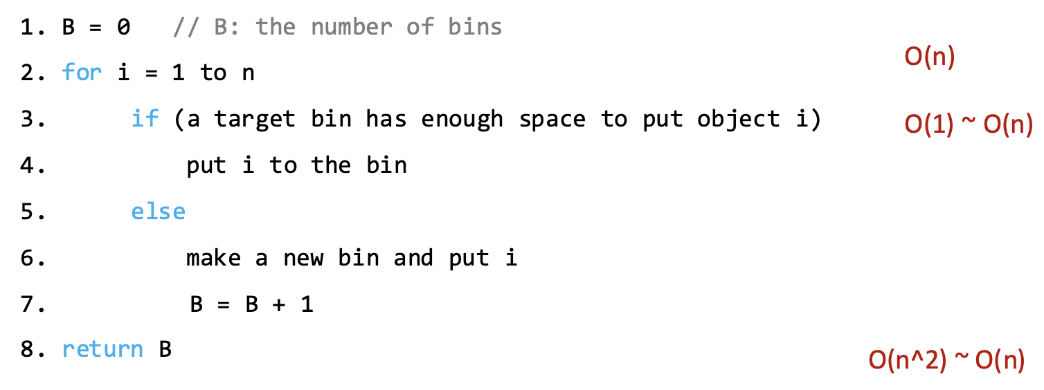
8.3.2 Approx_BinPacking()

• Input: n objects with their volumes
• Output: the number of used bins
• B: the number of bins

8.3.3 Appoximation Ratio

Lower bound of optimal solutions

• C: bin capacity
• V: sum of all volumes of objects
• M: the minimum number of bins (lower bound)
• M': the number of bins in an optimal solution

• M = V / C
• M <= M'

Lower bound of used bins for optimal solutions

• In greedy algorithms, using the first, best, or worst fit strategies
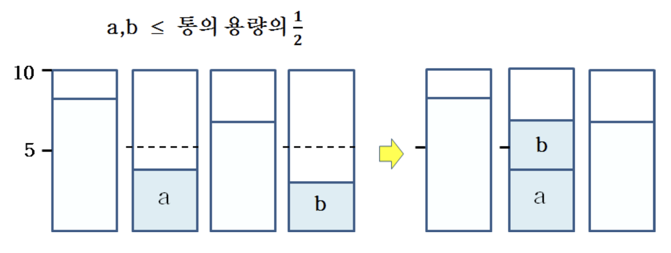
• Appoximated solutions should have 0 or 1 bin with less than C/2
• If is has more than 2 bins less than C/2
• When putting the object to make the second half-filled bin, the algorithm should have merged it with the first half-filled bin
• Two cases
  • 0 half-empty bin
    • Average volumes of products in all bins > C/2
  • 1 half-empty bin
    • Average volumes of products in (all bins - 1) > C/2

어떤 bin이 C/2 미만으로 채워져 있는데 또 다른 bin도 C/2 미만이라면, 그 둘을 합쳐도 C를 넘지 않으므로 greedy 과정에서 합쳐 하나의 bin으로 만들 수 있었어야 한다. 단, Next Fit은 제외한다.

Approximation Ratio

• Lower bound of used bins for optimal solutions
• M: the minimum number of bins(lower bound)
• M': the number of bins in an optimal solution
• M": the number of used bins of the optimal solution in the greedy algorithm(approximation)
• C / 2 < total volume/M" < total volume/(M"-1) (for any cases)
• (M"-1)/2 < (total volume/C = M) < M'
• (M"-1) < 2M'
• M" <= 2M' (by using natural number of M" and M'
• M"/M' <= 2

Approximation Ratio: "next fit"

• M: the number of used bins of the optimal solution in the greedy algorithm
• M': the optimal
• Total volume / C < M
• Total volume > M' / 2 * C
• M / M' < 2