9.0 Search Algorithm
Strategy
- Too complex problem
- No polynomial time algorithm
Approximation Proof
- Too exhaustive and not very useful
- Difficult to generalize
- Difficult to design for each different problem and conditions
What is the general approach to find a solution applicable to any problem?
Search the optimal solution
Process
- Set a candidate solution space
- Search a better solution
- Repeat until we can not find a better solution anymore
9.1 Backtracking
Idea
- A general serach method
- You can apply it to any optimization and decision problem
- The simplest search?
- Brute-Force inefficient
- Better Serach?
- If it's clear that a solution is not the optimum before evaluating its final quality
- (early) STOP evaluating the solution
Early Stopping은 search space size 자체를 pruning을 통해 줄이는 것이다.
9.1.1 Backtracking for TSP
- Memorize the best solution searched so far
- bestSolution = (cycle, distance)
- cycle: sequence of nodes
- distance: weight sum of all edges used in the cycle
- cycle = [starting node]
- bestSolution = (cycle, )
9.1.2 BacktrackTSP(cycle)
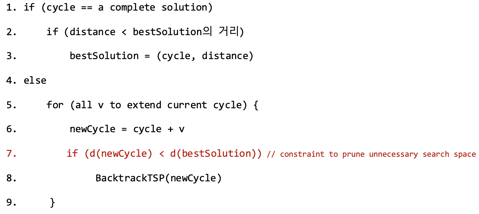
- Complete cycle이 구성되어야 bestSolution과 비교 및 업데이트가 가능하다.
Depth-First vs. Width-First
- Depth: 한 경로를 끝까지 탐색한 후 다른 경로로 이동
- 노드 추가 조건 검사 재귀 호출을 반복하며 트리의 깊이 방향으로 진행
- Width: 같은 레벨(깊이)의 모든 노드를 먼저 방문
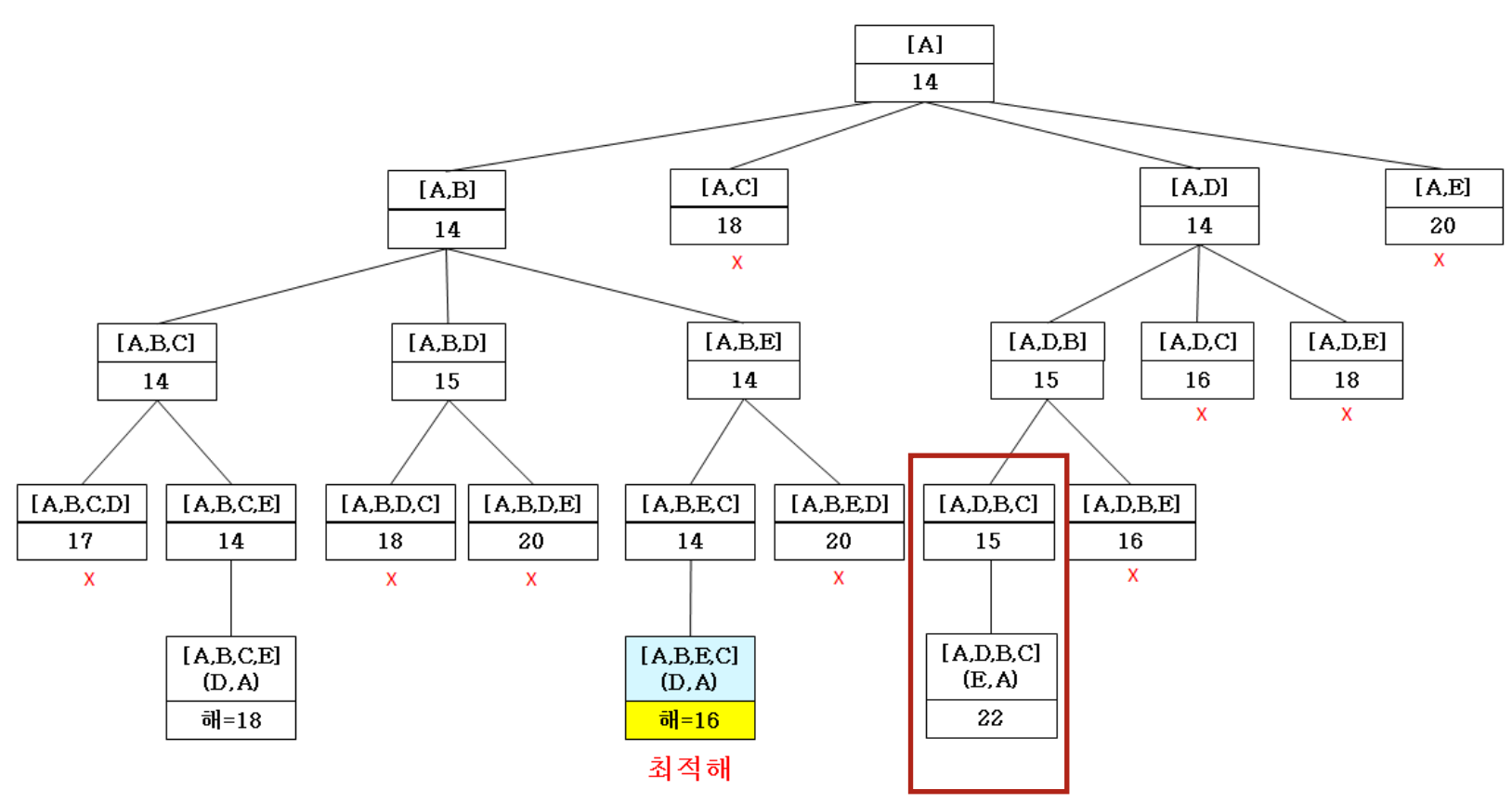
9.1.3 Procedure
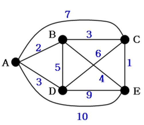
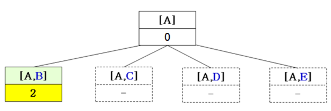
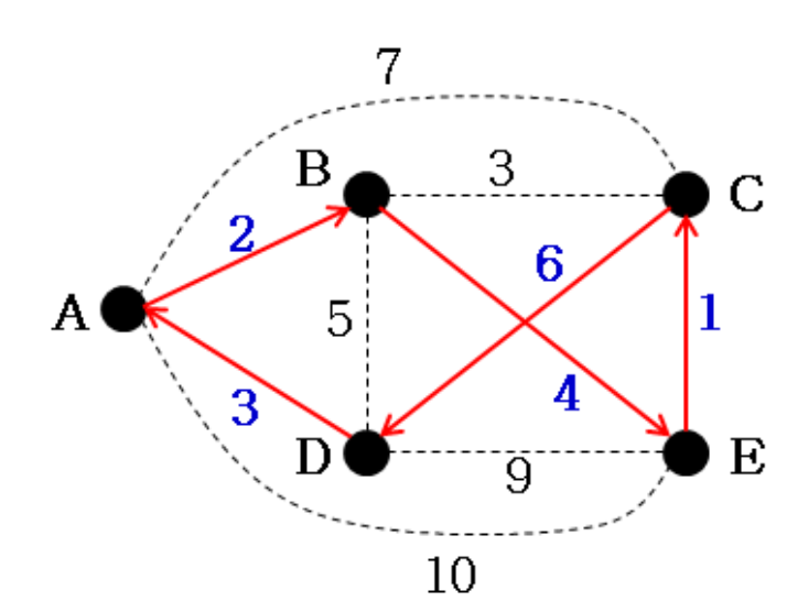
1. Starting node A
- cycle = [A]
- bestSolution = ([A], )
- Call BacktrackTSP(cycle)
2.
- Check new vertex to add to cycle [A]
- Candidate node {B, C, D, E}
- Check B first
- newcycle = [A, B]
- 후보 전부 선택이 가능하지만, while문 작동상으로 앞에 있는 B를 선택한다.
- d(newcycle) = 2(weight of (A, B))
3.
- Call BacktrackTSP([A, B])
- Depth First Search (by recursive call)
- Repeat until we find a complete solution
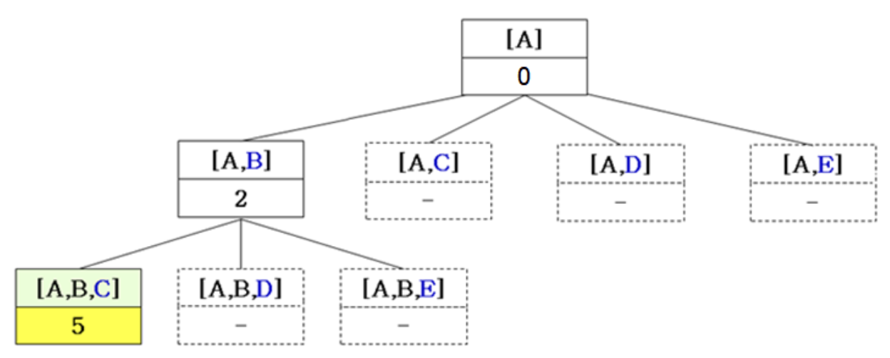
4. First terminated recursive all
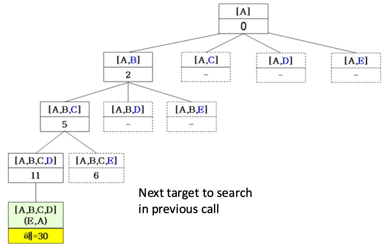
- 현재 경로: A B C D
- 남은 노드 E를 추가하고 다시 A로 돌아와 cycle 완성
- 현재 해에서 return하면 ABCE node로 이동, 이때 6 < 30이므로 진행
이때 비용이 30으로 계산되었고 이는 하나의 complete solution이므로 다른 후보들과 비교 가능한 상태가 된다.
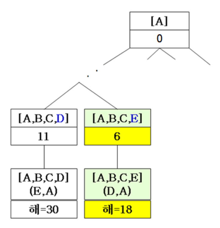
call stack mechanism
- ABC
- ABCD (먼저 탐색)
- ABCE (다음에 탐색할 대상)
5.
- bestSolution is updated to the second solution
- 18 < 30이므로 update
6.
- Intermediate results of running backtracking
call stack mechanism에 의해서 ABCEDA에서 return하면 부모인 AB의 다음 탐색 대상인 ABD로 return한다.
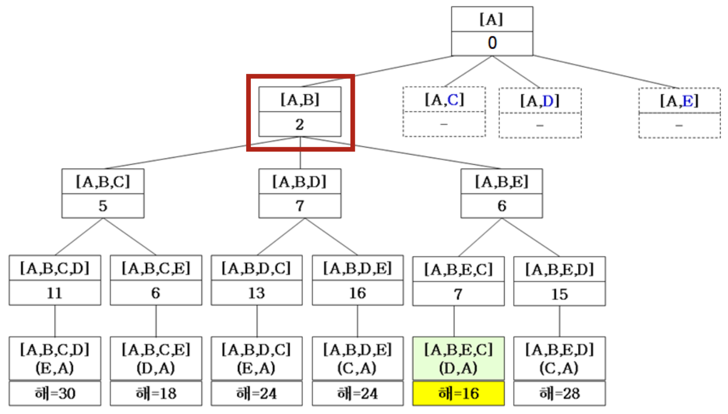
위 트리 구조에서는 아직까지 skip한 노드가 없다. Brute-Force
X
- no need to serach
- skip(pruning, early-stopping)
현재 bestSolution이 16, 비용이 16 이상 경로는 조기에 중단하여 계산량을 절감한다.
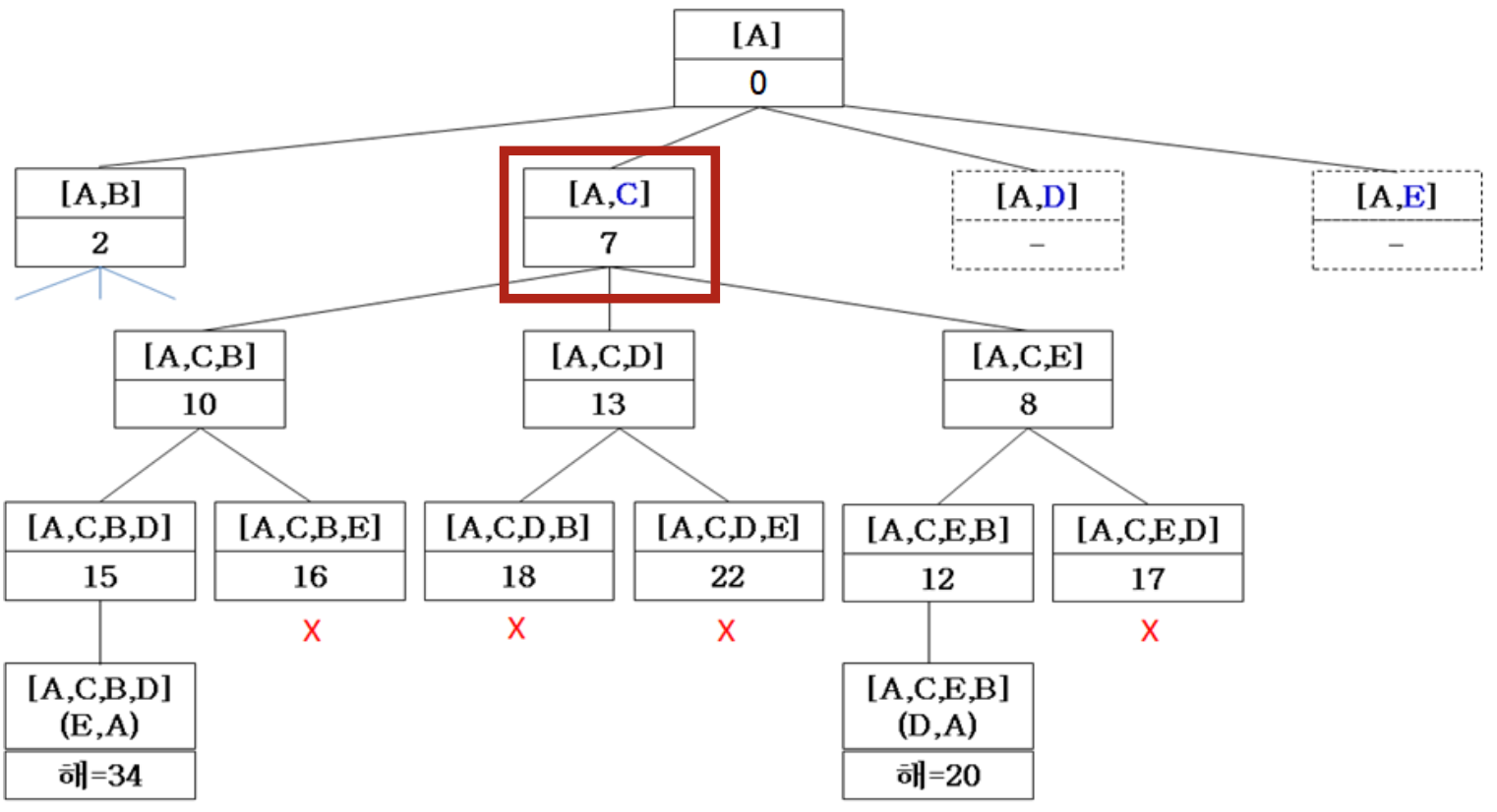
7. Brute-Force

9.1.4 Solution
- Final Solution = [A, B, C, E, D, A] with distance 16
- We checked all candidate solution
- Backtraking guarantees the optimal solution
- Faster than Brute-and-Force
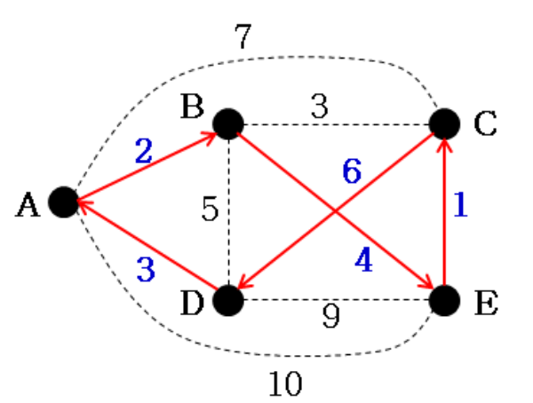
- Pruning을 통해 Bure-Force보다 효율적이지만, worse case의 겨우 Brute-Force 수준으로 퇴화한다.
- 최적해가 될 수 없는 경로만 배제하므로 본질적으로 전수조사로 분류할 수 있다.
9.1.5 Time Complexity
- Brute-Force Search: combinations or permutation of states
- Backtracking: a bit faster, but still
- States we can select in building a solution <= C
- Number of states to build a complete solution = n
- - Exponential time == Exhaustive Search
- C: 각 단계에서 선택 가능한 상태의 수
- n: 완전한 해를 만들기 위해 필요한 선택 단계의 수
시간 편차가 존재하지만, worst case는 거의 Brute-Force이다.
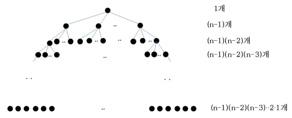
TSP problem에서는 이 더 정확한 표현이지만, 지수 시간이라는 의미에서는 과 같은 범주로 이해할 수 있다.
9.2 Branch-and-Bound
- Backtracking: depth first search
- Brute-Force, backtracking: so slow (exponential)
- Still exhaustive
- How to make search faster?
- Search most probable space first
- Simple strategy: quality estimation of each state Branch-and-Bound
Backtracking보다 빠르게 탐색하기 위해, 매 단계에서 퀄리티가 높은 상태부터 탐색하자.
Idea
- Quality estimation
- Search the most probable solutions first
- Skip most of bad solutions
- Faster than backtracking
- Best First Search
Branch-and-Bound는 Backtracking의 DFS 대신 Best-Fit Search를 사용해 추정값이 가장 높은 노드부터 탐색한다.
9.2.1 BranchAndBound(S)
- activeNodes: weight sum
- S: state, node
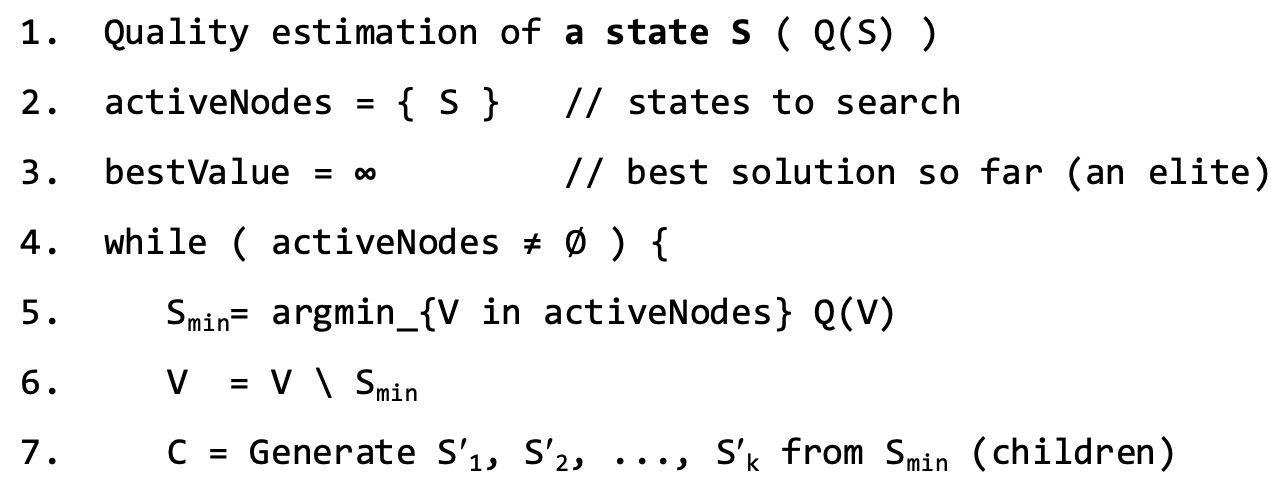
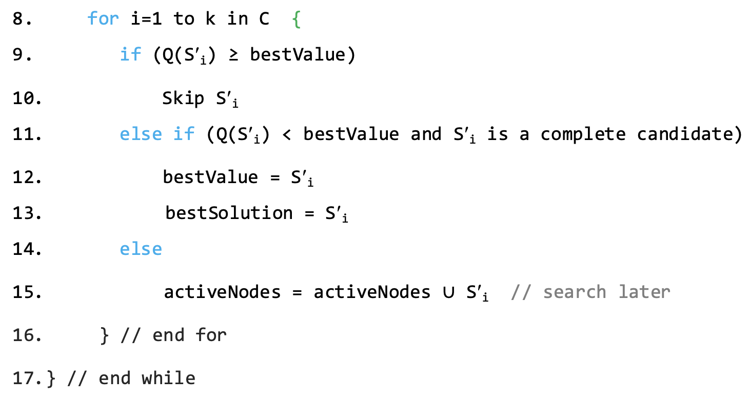
- activeNodes 중에서 Q(v)가 가장 좋은 상태를 하나 고르므로 Best-First Search에 해당한다.
BFS처럼 확장되지 않은 노드들의 집합을 한 곳에 모아두고 하나씩 확장한다. BFS는 Queue로 들어온 순서대로 꺼내지만, Branch-and-Bound의 Best-First는 우선순위 큐를 써서 bound(quality)가 가장 좋은 노드를 먼저 꺼낸다.
9.2.2 Quality Estimation
Idea
- All nodes in a TSP cycle have one input and one ouput edge
- Q(node) = + / 2
- Not correct in some cases
- Best Q(node) != selected edges in the optimal solution
- Rough Estimation
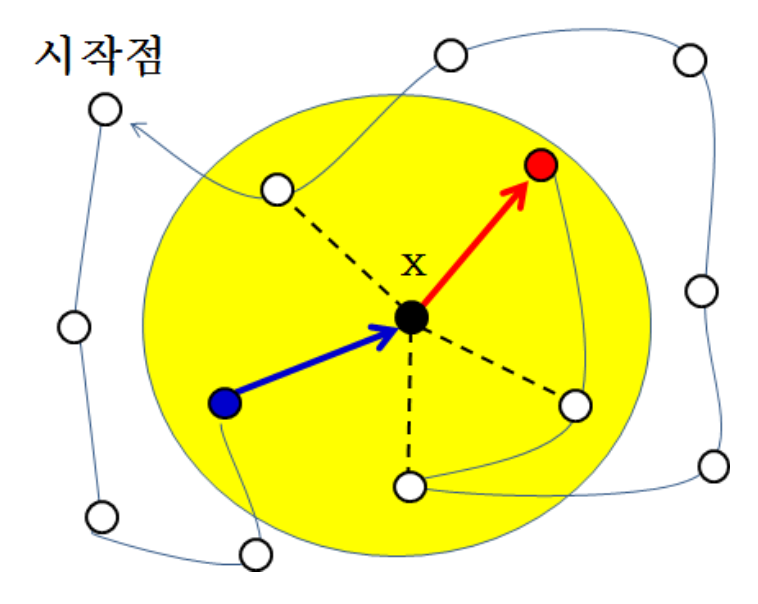
Fully conected니까 어떤 정점을 보아도 edge가 2개 이상 존재한다.
E.g., Quality Estimation
- May not be always correct
- But in many cases, it will be consistent to th edges to visit the node used in an optimum

TSP에서 하나의 cycle을 생성하려면, 각 노드마다 들어오는 간선과 나가는 간선을 하나씩 선택해야 한다. 이때 각 노드에서 weight가 가장 작은 in/out 간선을 우선적으로 선택하면 전체 path의 길이가 최소가 될 가능성이 커진다.
9.2.3 Branch-and-Bound for TSP
- A = Starting Node
- S = [A]
- Call Branch-and-Bound([A])
각 노드의 입장에서 퀄리티가 가장 좋은 edge를 2개씩 찾는다.
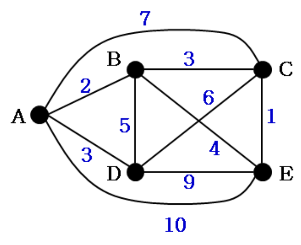
Initial Quality
- Sum of Q(each node)
- A: 2, 3
- B: 2, 3
- C: 1, 3
- D: 3, 5
- E: 1, 4
1.
- 각 정점에 대해 cycle 제약을 고려하지 않고 in/out의 최소 거리 합을 구해 TSP 경로의 Lower bound 계산
- E.g., 모든 정점에 대해 합산한 값이 27이므로 27/2 = 13.5, 14(올림 처리)
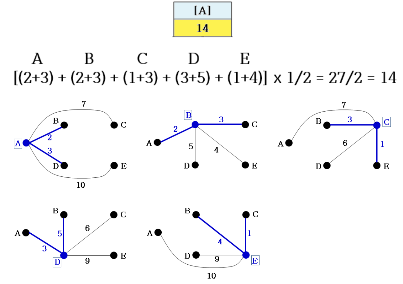
- Initialize activeNodes = {S}, bestValue =
- Select one state from acticeNodes
- ActiveNodes = {} // A를 선택하여 S에 넣어 공집합됨
- C = children of A
- {[A, B], [A, C], [A, D], [A, E]} // state representation = a path to nodes
- Evaluate their quality
2.
- Results after quality evaluation
- Quality of initial edge sets: 14 (not a complete solution)
- [A, B]: A B is fixed. Update Q(A) and Q(B) (no change in this exmaple)
- [A, C]: A C is fixed. Q(A) = 2+3/2 2+7/2, Q(C) = 2 4, total + 4
3.
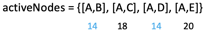
A에서 뻗어나갈 수 있는 노드 중 best는 B, E이므로 while문 구조상 B가 선택된다.
- Add all nonterminating nodes to activeNodes
- All nodes do not terminate
- Select = [A, B]
- Remove [A, B] from activeNodes
- activeNodes = {[A, C], [A, D], [A, E]}
- C = children of [A, B]
- Repeat
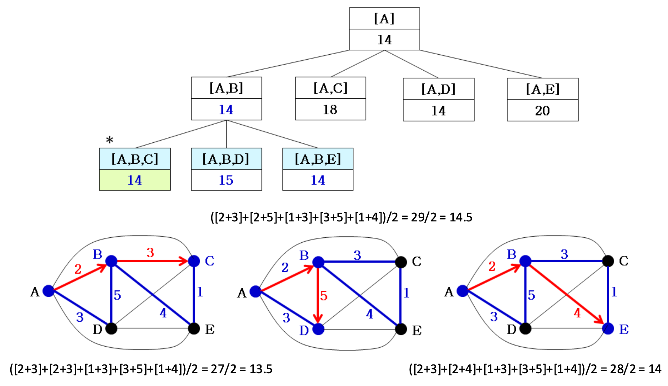
4.
Width + Best-Fit 방식으로 계속 진행된다.
5.
- [A, B, D]의 경우 14보다 큰 해이므로 skip
6.
- Update the best solution
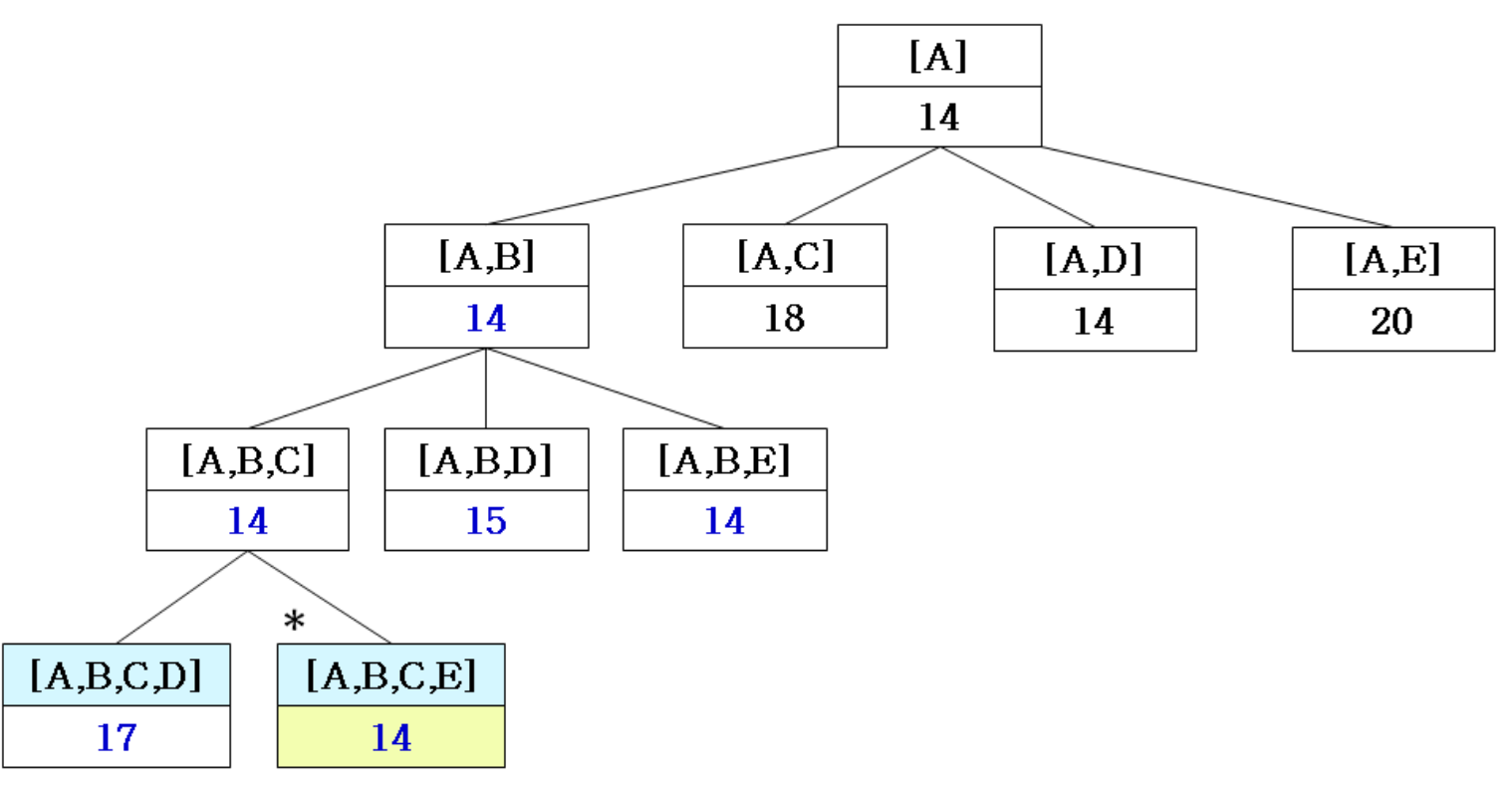
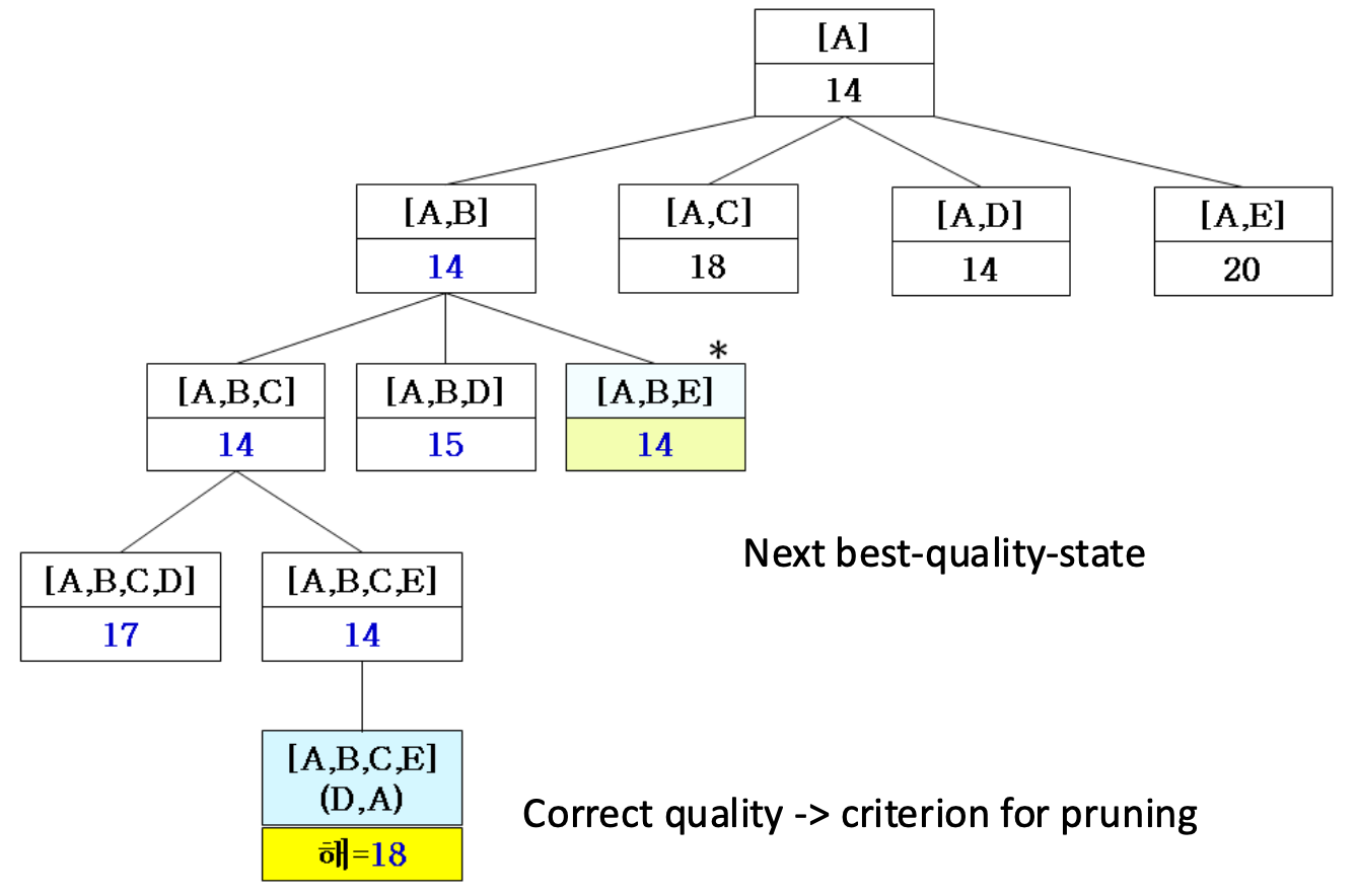
7. Best Solution [A, B, E, C, D, A] = 16
Traversed states
- Backtracking: 51
- Branch-and-Bound: 22
- Find a good criterion faster search