선형회귀 알고리즘 :: 경사하강법과 오차역전파

• 사이킷런, datasets 모듈에서 load_diabetes 패키지 임포트

• matpoltlib.pyplot 모듈 임포트

  	```

  from sklearn.datasets import load_diabetes
  import matplotlib.pyplot as plt

사이킷런 모듈의 당뇨병 환자 데이터 로드

• diabetes : bunch 데이터 타입 ... 일단 dict 타입과 동일하다고 봐도 무방
• data: 입력데이터, target: 타깃데이터

머신러닝 데이터 구조

• shape : 을 통해 넘파이 배열 크기 확인
• print(diabetes.data.shape) => (442, 10) :: 442행 10열의 2차원 배열. 442개의 샘플과 10개의 특성으로 이루어진 데이터
• print(diabetes.target.shape) => (442, ) :: 442개의 1차원 배열. 입력데이터의 샘플과 1:1 대응

    diabetes = load_diabetes()
    diabetes.data[0:3] # 배열 슬라이싱 샘플 0 1 2 뽑아내기
    diabetes.target[:3] # 배열 슬라이싱 샘플 0 1 2 뽑아내기
    
    print(diabetes.data.shape, diabetes.target.shape)

(442, 10) (442,)

산점도 출력

• plt.scatter( [x축 데이터배열], [y축 데이터 배열] ) 산점도 출력
• 입력데이터의 3번째 특성과 그에 대한 타깃데이터로 산점도 출력
• x축 diabetes.data 세번째 특성, y축 diabetes.target
• diabetes.data[:,2] 의미 => 샘플 첨부터 끝까지 3번째 특성을 자른다.
• plt.scatter(diabetes.data[:45,2], diabetes.target[:45])
  => x: 입력데이터의 44번째 샘플까지 3번 특성, y: 타깃데이터의 44개 데이터

    plt.scatter(diabetes.data[:,2], diabetes.target)
    # plt.scatter(diabetes.data[0:45,2], diabetes.target[0:45])
    x = diabetes.data[0:45,2]
    y = diabetes.target[0:45]
    plt.scatter(x,y)

<matplotlib.collections.PathCollection at 0x20993fc0bc8>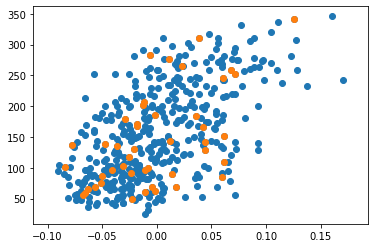

훈련 실습데이터 준비

-> 모델 훈련을 위한 '핵심 최적화 알고리즘'인 '경사하강법(gradientdescent)'에 대해 학습
-> 1개의 뉴런으로 구성된 첫 번째 모델 생성까지.

x = diabetes.data[:,2]
y = diabetes.target
plt.scatter(x,y)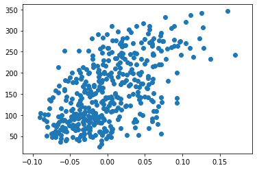

경사하강법 학습

선형회귀와 경사 하강법의 관계

• 선형회귀의 목표 : 입력 데이터(x)와 타깃 데이터(y)를 통해 기울기(a)와 절편(b)을 찾는 것
• 그렇게 찾아낸 y= ax + b 를 모델이라고 함
• 찾아낸 위의 모델, 즉 직선의 방정식이 회귀 알고리즘의 목표였고, 경사 하강법이 바로 이 목표를 달성하기 위한 방법 중 하나이다.
• 경사하강법 : 모델이 데이터를 잘 표현할 수 있도록, 기울기(변화율)를 사용하여 모델을 조금씩 조정하는 최적화 알고리즘

예측값과 변화율

• y^ = wx + b (vs y = ax + b)
• y^ : 예측값, w : 가중치
• 예측값으로 올바른 모델 찾기
  • 임의로 w, b 정하기
  • 샘플의 x 값에 따라 예측값 뽑아내기
  • 예측값과 샘플의 y값 비교
  • 예측값이 y 값과 가까워지도록 w,b조정.
  • 위 과정 반복

타깃와 예측 데이터 비교

    w = 1.0
    b = 1.0
    y_hat = x[0]*w + b
    print(y_hat, y[0], sep=" / ")

1.0616962065186886 / 151.0

w값 조절하여 예측값 바꾸기

    w_inc = w + 0.1
    y_hat_inc = x[0]*w_inc + b
    print(y_hat_inc, y[0], sep=" / ")

1.0678658271705574 / 151.0

값 조정 후 예측값 증가 정도 확인하기

    w_rate = (y_hat_inc - y_hat)/(w_inc - w)
    print(w_rate)

0.061696206518688734

변화율로 가중치 업데이트하기

    w_new = w + w_rate
    print(w_new)

1.0616962065186888

변화율로 절편 업데이트하기

• 아래의 결과를 보면 절편의 변화율은 1이다.
• 즉 b가 1이 증가하면 y_hat도 1만큼 증가한다.
• 즉 b를 업데이트하기 위해서는 변화율이 1이므로 단순히 1을 더하면 된다.

    b_inc = b + 0.1
    y_hat_inc = x[0]*w + b_inc
    
    b_rate = (y_hat_inc - y_hat)/(b_inc - b)
    print(b_rate)

	1.0

오차역전파로 가중치와 절편을 더 적절하게 업데이트한다.

• 위의 예처럼 가중치와 절편을 업데이트 하는 방법은 수동적인 방법이다.
• 오차 역전파 : 오차가 연이어 전파되는 모습으로 수행.
• y에서 y^을 뺀 오차의 양을 변화율에 곱하는 방법으로 w를 업데이트한다. 이렇게 하면 y^이 y보다 많이 작은 경우, w와 b를 많이 바꿀 수 있다. 또한 y^이 y를 지나치면 w와 b의 방향을 바꿔준다.

    err = y[0] - y_hat
    w_new = w + w_rate*err
    b_new = b + 1*err
    print(w_new, b_new)

10.250624555904514 150.9383037934813

    y_hat = x[1]*w_new + b_new
    err = y[1] - y_hat
    w_rate = x[1]
    w_new = w_new + w_rate*err
    b_new = b_new + 1*err
    print(w_new, b_new)

14.132317616381767 75.52764127612664

전체 샘플 반복하기

• zip() 함수는 여러 배열에서 요소를 하나씩 꺼내서 사용할 수 있도록 해준다.

    x = diabetes.data[:,2]
    y = diabetes.target
    for x_i, y_i in zip(x,y):
        y_hat = x_i*w + b
        err = y_i - y_hat
        w_rate = x_i
        w = w + w_rate*err
        b = b + 1*err
    print(w,b)

587.8654539985689 99.40935564531424

직선함수 그리기

• 시작점의 좌표와 종점의 좌표를 plot() 함수에 인자로 전달한다.

    plt.scatter(x,y)
    pt1 = (-0.1, -0.1*w+b)
    pt2 = (0.15, 0.15*w + b)
    plt.plot( [pt1[0],pt2[0]], [pt1[1],pt2[1]] )
    plt.xlabel('x')
    plt.ylabel('y')
    plt.show()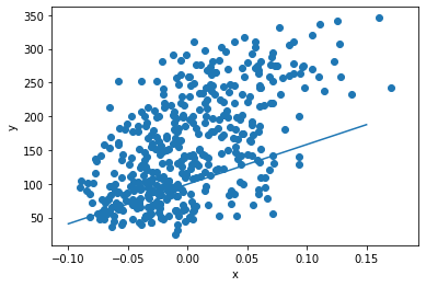

여러 에포크를 반복한다

• 위의 직선그래프는 산점도의 흐름과 약간 빗나가는 것을 알 수 잇다.
• 보통 경사하강법에서는 주어진 훈련데이터로 학습을 여러 번 반복하며, 이렇게 전체 훈련 데이터를 모두 이용하여 한 단위의 작업을 진행하는 것을 에포크(epoch)라고 한다. 수십에서 수천번을 반복한다.
• 우리가 해야할 것은 바깥에 for문을 한번 더 씌우는 것 뿐이다.
• 100 에포크를 돌리고 업데이트 된 w, b를 이용해 직선도를 출력해보면 위의 그래프보다 정확한 것을 알 수 있다.

    for i in range(1, 100):
        for x_i, y_i in zip(x,y):
            y_hat = x_i*w + b
            err = y_i - y_hat
            w_rate = x_i
            w = w + w_rate*err
            b = b + 1*err
    print(w,b)

913.5973364345905 123.39414383177204

    plt.scatter(x,y)
    pt1 = (-0.1, -0.1*w+b)
    pt2 = (0.15, 0.15*w + b)
    plt.plot( [pt1[0],pt2[0]], [pt1[1],pt2[1]] )
    plt.xlabel('x')
    plt.ylabel('y')
    plt.show()

머신러닝 모델 추출

									`y^ = 913.6x + 123.4`

• 새로운 모델로 값을 예측해볼 수 있게 되었다
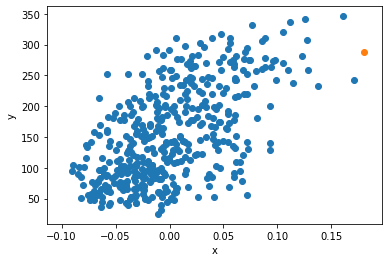
• 입력데이터 x에 없었던 새로운 데이터를 통해 예측값을 구해볼 수 있다.

    x_new = 0.18
    y_pred = x_new*w+b
    print(y_pred)

    287.8416643899983

    plt.scatter(x,y)
    plt.scatter(x_new,y_pred)
    plt.xlabel('x')
    plt.ylabel('y')
    plt.show()