ZeroR, OneR, Naive Bayes Classifier
실습 내용:
-
ZeroR
-
OneR
-
Naive Bayes classifier
import numpy as np
import pandas as pd
import sklearn
print(sklearn.__version__)1.0.2
실습 데이터
# 데이터 받기
url = "https://raw.githubusercontent.com/inikoreaackr/ml_datasets/main/playgolf.csv"
df = pd.read_csv(url)
# 데이터 첫 다섯 instance 확인
df.head()| OUTLOOK | TEMPERATURE | HUMIDITY | WINDY | PLAY GOLF | |
|---|---|---|---|---|---|
| 0 | Rainy | Hot | High | False | No |
| 1 | Rainy | Hot | High | True | No |
| 2 | Overcast | Hot | High | False | Yes |
| 3 | Sunny | Mild | High | False | Yes |
| 4 | Sunny | Cool | Normal | False | Yes |
# 데이터 타입 확인
df.dtypes
OUTLOOK object TEMPERATURE object HUMIDITY object WINDY bool PLAY GOLF object dtype: object
# object 타입을 category로 변경
for col in df.columns:
  df[col] = df[col].astype('category')
# 변경이 되었는지 확인
df.dtypesOUTLOOK category TEMPERATURE category HUMIDITY category WINDY category PLAY GOLF category dtype: object
1. ZeroR
ZeroR은 가장 간단한 분류 방법이며, 다른 모든 feature들을 무시하고 label에만 의존합니다.
ZeroR 분류기는 단순히 데이터의 class를 다수 카테고리로 예측합니다.
ZeroR에는 예측 능력이 없지만, 이것은 표준 성능을 가늠하여 다른 분류 방법 성능의 기준점이 됩니다.
# PLAY GOLF feature 출력
df['PLAY GOLF']
0 No 1 No 2 Yes 3 Yes 4 Yes 5 No 6 Yes 7 No 8 Yes 9 Yes 10 Yes 11 Yes 12 Yes 13 No Name: PLAY GOLF, dtype: category Categories (2, object): ['No', 'Yes']
# PLAY GOLF는 binary 변수입니다. 각 카테고리의 갯수를 세어봅니다.
df['PLAY GOLF'].value_counts(sort = True)
Yes 9 No 5 Name: PLAY GOLF, dtype: int64
# 이 데이터셋에서 "Play Golf = Yes"로 예측하는 ZeroR 모델의 정확도를 계산해봅니다.
9 / (9 + 5)
0.6428571428571429
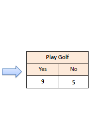
위의 데이터셋에서 "Play Golf = Yes"로 예측하는 ZeroR모델의 정확도는 0.64가 됩니다.
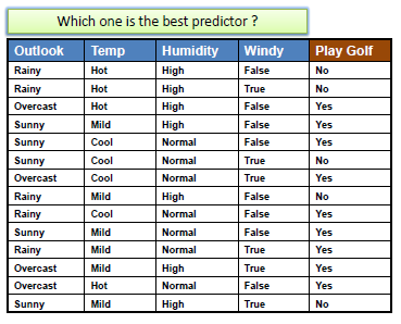
OneR
OneR은 One Rule의 약자이며, 간단하고 정확한 분류 알고리즘입니다.
OneR은 데이터의 각 feature 마다 하나의 룰 셋(Rule Set)을 생성합니다. 그리고 생성된 룰 셋 중에서, 전체데이터에 대해 오차가 가장 작은 룰 셋을 One Rule로 결정합니다.
각 feature당 룰 셋은 frequency table을 이용하여 만들 수 있습니다.
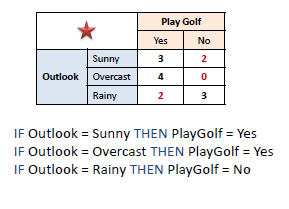
OneR Algorithm
각 feature 마다,

    각 feature의 value 마다, 룰을 아래와 같이 만듭니다.

        그 feature의 value에 해당되는 instance중에 target class가 몇개인지 셉니다.

        가장 갯수가 많은 class를 찾습니다.

        그 feature의 value가 해당되면 그 갯수가 많은 class로 예측되도록 룰을 하나 만듭니다.

    각 feature의 룰들의 전체 에러를 계산합니다. (반대로 정확도를 계산할 수도 있습니다.)

가장 작은 에러를 보이는 feature을 선택합니다.
아래 그림에서는 outlook과 humidity feature 모두 에러의 갯수가 4이므로 제일 작습니다. 하지만 활동에서는 첫번째 feature인 outlook만 고려할 것입니다.
For example:
# 수도코드 구현
from collections import Counter

total_errors = []

for col in df.columns[:-1]:
  error = 0
  for val in df[col].unique():
    length = len(df[df[col] == val])
    print(f"{col} : {val}, length : {length}")
    print(Counter(df[df[col] == val]['PLAY GOLF']).most_common())
    error += (length - Counter(df[df[col] == val]['PLAY GOLF']).most_common()[0][1])
  print(f"\nerror of {col}: [{error}] \n")
  total_errors.append(error)
OUTLOOK : Rainy, length : 5
[('No', 3), ('Yes', 2)]
OUTLOOK : Overcast, length : 4
[('Yes', 4)]
OUTLOOK : Sunny, length : 5
[('Yes', 3), ('No', 2)]
error of OUTLOOK: [4]
TEMPERATURE : Hot, length : 4
[('No', 2), ('Yes', 2)]
TEMPERATURE : Mild, length : 6
[('Yes', 4), ('No', 2)]
TEMPERATURE : Cool, length : 4
[('Yes', 3), ('No', 1)]
error of TEMPERATURE: [5]
HUMIDITY : High, length : 7
[('No', 4), ('Yes', 3)]
HUMIDITY : Normal, length : 7
[('Yes', 6), ('No', 1)]
error of HUMIDITY: [4]
WINDY : False, length : 8
[('Yes', 6), ('No', 2)]
WINDY : True, length : 6
[('No', 3), ('Yes', 3)]
error of WINDY: [5]
# 오류가 가장 작은 feature를 고릅니다.

best_feature = df.columns[np.argmin(total_errors)]
print(best_feature)
OUTLOOK
# best feature에 대해 룰셋을 생성합니다.
oneRules = []
for val in df[best_feature].unique():
  print(f"{best_feature} : {val}", "-> ", end = ' ')
  print(Counter(df[df[best_feature] == val]['PLAY GOLF']).most_common()[0][0])
  oneRules.append((best_feature, val, Counter(df[df[best_feature] == val]['PLAY GOLF']).most_common()[0][0]))
OUTLOOK : Rainy -> No OUTLOOK : Overcast -> Yes OUTLOOK : Sunny -> Yes
The best feature is:
Naive Bayes Classifier with scikit-learn
- scikit-learn의 Naive Bayes classifier 다큐멘테이션: https://scikit-learn.org/stable/modules/naive_bayes.html
df.head()| OUTLOOK | TEMPERATURE | HUMIDITY | WINDY | PLAY GOLF | |
|---|---|---|---|---|---|
| 0 | Rainy | Hot | High | False | No |
| 1 | Rainy | Hot | High | True | No |
| 2 | Overcast | Hot | High | False | Yes |
| 3 | Sunny | Mild | High | False | Yes |
| 4 | Sunny | Cool | Normal | False | Yes |
df.describe()| OUTLOOK | TEMPERATURE | HUMIDITY | WINDY | PLAY GOLF | |
|---|---|---|---|---|---|
| count | 14 | 14 | 14 | 14 | 14 |
| unique | 3 | 3 | 2 | 2 | 2 |
| top | Rainy | Mild | High | False | Yes |
| freq | 5 | 6 | 7 | 8 | 9 |
# 카테고리 데이터를 정수로 인코딩
df_enc = pd.DataFrame()
df_enc['OUTLOOK'] = df['OUTLOOK'].cat.codes
df_enc['TEMPERATURE'] = df['TEMPERATURE'].cat.codes
df_enc['HUMIDITY'] = df['HUMIDITY'].cat.codes
df_enc['WINDY'] = df['WINDY'].cat.codes
df_enc['PLAY GOLF'] = df['PLAY GOLF'].cat.codesdf_enc.head()| OUTLOOK | TEMPERATURE | HUMIDITY | WINDY | PLAY GOLF | |
|---|---|---|---|---|---|
| 0 | 1 | 1 | 0 | 0 | 0 |
| 1 | 1 | 1 | 0 | 1 | 0 |
| 2 | 0 | 1 | 0 | 0 | 1 |
| 3 | 2 | 2 | 0 | 0 | 1 |
| 4 | 2 | 0 | 1 | 0 | 1 |
</div># 인코딩된 데이터의 타입을 프린트해봅니다.
df_enc.dtypesOUTLOOK int8 TEMPERATURE int8 HUMIDITY int8 WINDY int8 PLAY GOLF int8 dtype: object
# 분류기에 넣을 feature과 해당 label을 구분합니다.
features = df_enc.drop(columns=['PLAY GOLF'])
label = df_enc['PLAY GOLF']
from sklearn.naive_bayes import CategoricalNB
model = CategoricalNB()model.fit(features.values, label)CategoricalNB()
score = model.score(features.values, label)
score
0.9285714285714286
# p(x_i|y_i) 출력
from pprint import pprint
feature_log_prior = model.feature_log_prob_
for feature_prior in feature_log_prior:
  pprint(np.exp(feature_prior))
array([[0.125 , 0.5 , 0.375 ],
[0.41666667, 0.25 , 0.33333333]])
array([[0.25 , 0.375 , 0.375 ],
[0.33333333, 0.25 , 0.41666667]])
array([[0.71428571, 0.28571429],
[0.36363636, 0.63636364]])
array([[0.42857143, 0.57142857],
[0.63636364, 0.36363636]])
# p(y_j) 출력
np.exp(model.class_log_prior_)
array([0.35714286, 0.64285714])
# instances에 대해서 예측을 해봅니다.
# ("Sunny", "Hot", "Normal", False) [2, 1, 1, 0]
# ("Rainy", "Mild", "High", False) [1, 2, 0, 0]

print(model.predict_proba([[2, 1, 1, 0]]), model.predict([[2, 1, 1, 0]]))
print(model.predict_proba([[1, 2, 0, 0]]), model.predict([[1, 2, 0, 0]]))
[[0.22086561 0.77913439]] [1] [[0.5695011 0.4304989]] [0]
1. 기계학습 기본 용어 정의/의미
- 기계학습: 인공지능의 한 분야로 사람의 학습과 같은 능력을 컴퓨터를 통해 실현하고자 하는 기술로, 데이터로부터 모델을 만들어내는 과정을 의미한다.
- Label (=target): label은 model이 예측하려는 값으로 training을 한 후의 output이다. 데이터를 차별화 할 수 있는 범주이다.
- class: 데이터를 분류하는 범주
- Features: feature은 training data의 분석 대상이 되는 속성들로 input set에 있는 column으로 표현된다.
- Input: input은 일반적으로 model에 전당되는 데이터 집합(X)를 나타낸다. 예를 들어 (X,Y(label)) 형태의 데이터 세트에서 X는 입력이며 레이블인 Y는 대상 또는 출력이 된다.
- Numerical data (=Quantitative data): Numerical data는 숫자로 표현되는 것을 의미한다.
- Categorical data
(=Qualitative data): Categorical data는 일반적으로 숫자로 표현되지 않는 것을 의미하며 이산적인 형태의 데이터를 표현하기 위해 사용된다.
- Unlabeled example (=instance): Unlabeled example은 주로 unsupervised learning에 사용되는 데이터로 의미 있는 label이 존재하지 않는다. training data의 한 예시로 예상되는 결과에 대해 정보를 내포하지 않은 데이터이다.
- Labeled example:labeled example은 주로 supervised learning에 사용되는 데이터로 의미 있는 label이나 class를 가지고 있다.
- Training (=learning): 주로 성능의 향상을 의미한다. 경험(data)에 따라 예측하려는 값에 대해 배우는 것으로 명시적인 지시가 아닌 경험에 의해 작업의 성능이 향상되는 것을 의미한다.
- Predict (=inference): prediction이란 과거의 data set에 대한 training을 거쳐 특정 결과의 가능성을 예측하는 model의 출력을 의미한다.
- Train Set: Train set은 기계 학습 model을 훈련하는데 사용되는 데이터이다.
- Test Set: Test set은 학습된 모델을 테스트하기 위한 data의 하위 set이다.
- Regression: feature와 outcome 간의 관계를 이해하기 위한 방법으로 이를 통해 관계가 추정되면 결과를 예측할 수 있게 된다. 기계학습에서는 일반적으로 best fit을 그리는 작업을 의미하며 각 point 사이의 거리를 최소화하는 방법을 통해 best fit을 찾는다.
- Error (=loss): model의 오류 합계를 나타내는 값으로 model이 얼마나 잘 훈련되었는지를 판단한다. loss가 크면 model이 제대로 작동하지 않는다는 것을 의미한다.
- Classification: classification은 input의 주어진 data에 대하여 특정 class label을 예측하는 model을 의미한다.
- Accuracy: Accuracy는 model이 얼마나 잘 예측하고 있는지를 측정한다.
2. 적용 과제
Data documentation: Car Evaluation, Balloons
- Car Evaluation의 feature:
buying,maint,doors,persons,lung_boot,satefy
- Car Evalaution의 label:
accept
- Balloons의 feature:
color,size,act,age
- Balloons의 label:
inflated
2.1 pandas
- 아래 data url을 통해 각 데이터마다 dataframe을 생성합니다.
- Car Evalaution의 모든 column name을 출력하시오.
- Car Evaluation의
buyingfeature에 어떤 카테고리가 있는지 출력하시오.
- Car Evaluation의
acceptlabel의 각 class와 해당 class의 instance 개수를 메소드 하나로 출력하시오.
- Balloons에서
colorfeature이yellow인 instance을 모두 출력하시오.
# load data
car_url = 'https://archive.ics.uci.edu/ml/machine-learning-databases/car/car.data'
balloons_url = 'https://archive.ics.uci.edu/ml/machine-learning-databases/balloons/adult+stretch.data'
import numpy as np
import pandas as pd
import sklearn# 데이터 프레임 생성
car_df = pd.read_csv(car_url, header = None)
car_df.columns = ["buying", "maint", "doors", "persons", "lung_boot", "satefy", "accept"]
bal_df = pd.read_csv(balloons_url, header = None)
bal_df.columns = ["color", "size", "act", "age", "inflated"]# 데이터의 column name 출력
print(car_df.columns.to_list()[:-1])
print(bal_df.columns.to_list()[:-1])['buying', 'maint', 'doors', 'persons', 'lung_boot', 'satefy'] ['color', 'size', 'act', 'age']
# Car evaluation 'buying' feature 의 카테고리 출력

print(car_df['buying'].unique())
['vhigh' 'high' 'med' 'low']
# Car evaluation 'accept' label 의 각 class 와 instance 개수

car_df['accept'].value_counts(sort = True)
unacc 1210 acc 384 good 69 vgood 65 Name: accept, dtype: int64
# Balloons에서 'color' feature이 yellow인 instance 출력

bal_df['color'].value_counts(sort = True)
print(bal_df.loc[(bal_df['color'] == 'YELLOW')])
color size act age inflated 0 YELLOW SMALL STRETCH ADULT T 1 YELLOW SMALL STRETCH ADULT T 2 YELLOW SMALL STRETCH CHILD F 3 YELLOW SMALL DIP ADULT F 4 YELLOW SMALL DIP CHILD F 5 YELLOW LARGE STRETCH ADULT T 6 YELLOW LARGE STRETCH ADULT T 7 YELLOW LARGE STRETCH CHILD F 8 YELLOW LARGE DIP ADULT F 9 YELLOW LARGE DIP CHILD F
2.2 데이터 이해 및 전처리
데이터 정보를 읽고 각 feature이 무슨 의미인지 파악하여 서술합니다. 실습했던 내용을 바탕으로 Car Evaluation 데이터와 Balloons 데이터를 scikit-learn의 Categorical Naive Bayesian Classifier에 적합하도록, Object 타입을 정수형으로 전처리합니다.
2.3 모델 생성, 훈련 및 결과 해석
scikit-learn 패키지를 사용하여 car와 balloons 두 데이터에:
-
Categorical Naive Bayesian Classifier을 fit합니다.
-
두 데이터에 대하여 score를 출력합니다.
-
각 class probability와 각 feature probability을 출력합니다.
-
본인이 임의로 만든 두개의 각기 다른 instances에 대하여 예측을 출력합니다. (car 두 개, balloons 두 개, 총 네 개)
-
모델 예측 결과를 데이터의 맥락으로 해설합니다. (ex. 자동차1의 가격이 높고 보수비용이 낮으며... 할 때, 모델은 자동차1의 평가를 매우 좋음으로 예측하였다.)
Car Evaluation의 feature: buying, maint, doors, persons, lung_boot, satefy
-
buying :차량의 구매 가격
-
maint : 차량을 유지보수하기 위한 가격
-
doors : 문의 개수
-
persons : 차량이 운반할 수 있는 사람의 수 (탑승인원)
-
lung_boot : 차량 트렁크의 크기
-
safety : 안전 측정에서 평가된 차량 안전
Car Evalaution의 label: accept
** accept 차량의 용인 가능성(구매 가능성)
Balloons의 feature: color, size, act, age
-
color : 풍선의 색상
-
size : 풍선의 크기
-
act : 풍선을 늘어나게 했는지 줄어들게 했는지 여부
-
age : 나이 / 어른 아이 여부
Balloons의 label: inflated
** inflated 풍선이 부풀려진 여부
# Object 타입을 정수형으로 전처리

car_df_enc = pd.DataFrame()
bal_df_enc = pd.DataFrame()

# Car evaluation
for col in car_df.columns:
  car_df[col] = car_df[col].astype('category')

car_df_enc['buying'] = car_df['buying'].cat.codes
car_df_enc['maint'] = car_df['maint'].cat.codes
car_df_enc['doors'] = car_df['doors'].cat.codes
car_df_enc['persons'] = car_df['persons'].cat.codes
car_df_enc['lung_boot'] = car_df['lung_boot'].cat.codes
car_df_enc['satefy'] = car_df['satefy'].cat.codes
car_df_enc['accept'] = car_df['accept'].cat.codes

# Balloons
for col in bal_df.columns:
  bal_df[col] = bal_df[col].astype('category')

bal_df_enc['color'] = bal_df['color'].cat.codes
bal_df_enc['size'] = bal_df['size'].cat.codes
bal_df_enc['act'] = bal_df['act'].cat.codes
bal_df_enc['age'] = bal_df['age'].cat.codes
bal_df_enc['inflated'] = bal_df['inflated'].cat.codes
from sklearn.naive_bayes import CategoricalNB
car_model = CategoricalNB()
bal_model = CategoricalNB()# Car evaluation fit & score 출력
car_features = car_df_enc.drop(columns=['accept'])
car_label = car_df_enc['accept']
car_model.fit(car_features.values, car_label)
car_score = car_model.score(car_features.values, car_label)
car_score0.8715277777777778
# Balloons fit & score 출력

bal_features = bal_df_enc.drop(columns=['inflated'])
bal_label = bal_df_enc['inflated']
bal_model.fit(bal_features.values, bal_label)
bal_score = bal_model.score(bal_features, bal_label)
bal_score
1.0
# class probability& feature probability 출력

# Car evaluation
from pprint import pprint

car_feature_log_prior = car_model.feature_log_prob_
for featue_prior in car_feature_log_prior:
  pprint(np.exp(featue_prior))
print(np.exp(car_model.class_log_prior_))
array([[0.28092784, 0.23195876, 0.29896907, 0.18814433],
[0.01369863, 0.64383562, 0.32876712, 0.01369863],
[0.26771005, 0.21334432, 0.22158155, 0.29736409],
[0.01449275, 0.57971014, 0.39130435, 0.01449275]])
array([[0.27319588, 0.23969072, 0.29896907, 0.18814433],
[0.01369863, 0.64383562, 0.32876712, 0.01369863],
[0.25947282, 0.22158155, 0.22158155, 0.29736409],
[0.20289855, 0.39130435, 0.39130435, 0.01449275]])
array([[0.21134021, 0.25773196, 0.26546392, 0.26546392],
[0.21917808, 0.26027397, 0.26027397, 0.26027397],
[0.2693575 , 0.24794069, 0.24135091, 0.24135091],
[0.15942029, 0.23188406, 0.30434783, 0.30434783]])
array([[0.00258398, 0.51421189, 0.48320413],
[0.01388889, 0.51388889, 0.47222222],
[0.47568013, 0.25803792, 0.26628195],
[0.01470588, 0.45588235, 0.52941176]])
array([[0.374677 , 0.35142119, 0.27390181],
[0.34722222, 0.34722222, 0.30555556],
[0.30420445, 0.32399011, 0.37180544],
[0.60294118, 0.38235294, 0.01470588]])
array([[0.52971576, 0.00258398, 0.46770026],
[0.43055556, 0.01388889, 0.55555556],
[0.22918384, 0.47568013, 0.29513603],
[0.97058824, 0.01470588, 0.01470588]])
[0.22222222 0.03993056 0.70023148 0.03761574]
# Balloons

bal_feature_log_prior = bal_model.feature_log_prob_
for featue_prior in bal_feature_log_prior:
  pprint(np.exp(featue_prior))
print(np.exp(bal_model.class_log_prior_))
# car evaluation instances 예측
# ("vhigh", "vhigh", 2, 2, "small", "high") [3, 3, 0, 0, 2, 0]
# ("low", "low", "5more", "more", "big, "med) [1, 1, 3, 2, 0, 0]
print(car_model.predict_proba([[3, 3, 0, 0, 2, 0]]), car_model.predict([[3, 3, 0, 0, 2, 0]]))
print(car_model.predict_proba([[1, 1, 3, 2, 0, 0]]), car_model.predict([[1, 1, 3, 2, 0, 0]]))[[9.21115137e-04 4.43484909e-06 9.99074059e-01 3.90721613e-07]] [2] [[0.20014669 0.19352277 0.09437552 0.51195502]] [3]
# balloons instances 예측
#("YELLOW","LARGE", "STRETCH", "ADULT") [1, 0, 1, 0]
#("PULPLE", "SMALL", "DIP", "ADULT") [0, 1, 0, 0]

print(bal_model.predict_proba([[1, 0, 1, 0]]), bal_model.predict([[1, 0, 1, 0]]))
print(bal_model.predict_proba([[0, 1, 0, 0]]), bal_model.predict([[0, 1, 0, 0]]))
[[0.19107307 0.80892693]] [1] [[0.79281184 0.20718816]] [0]
bal_df_enc.head(15)| color | size | act | age | inflated | |
|---|---|---|---|---|---|
| 0 | 1 | 1 | 1 | 0 | 1 |
| 1 | 1 | 1 | 1 | 0 | 1 |
| 2 | 1 | 1 | 1 | 1 | 0 |
| 3 | 1 | 1 | 0 | 0 | 0 |
| 4 | 1 | 1 | 0 | 1 | 0 |
| 5 | 1 | 0 | 1 | 0 | 1 |
| 6 | 1 | 0 | 1 | 0 | 1 |
| 7 | 1 | 0 | 1 | 1 | 0 |
| 8 | 1 | 0 | 0 | 0 | 0 |
| 9 | 1 | 0 | 0 | 1 | 0 |
| 10 | 0 | 1 | 1 | 0 | 1 |
| 11 | 0 | 1 | 1 | 0 | 1 |
| 12 | 0 | 1 | 1 | 1 | 0 |
| 13 | 0 | 1 | 0 | 0 | 0 |
| 14 | 0 | 1 | 0 | 1 | 0 |
모델 예측 결과 해설
car evaluation
자동차 3(index 2)는 가격이 매우 높고 보수 비용도 매우 높으며 차량의 문이 2개이고 탑승 가능 인원이 2명이다. 트렁크 크기는 작고, 안전평가에서 매우 높은 평가를 받았는데 모델은 자동차 3을 수용불가로 예측했다.
자동차 1728(index 1727) 가격이 낮고 보수 비용도 매우 낮으며 차량의 문은 5개 이상이고 인원도 이상이며 트렁크 크기가 크고 안전평가에서는 중간 단계의 평가를 받았다. 모델은 자동차 1728을 매우 좋음으로 예측하였다.
balloons
풍선 6(index5)는 노란색이고 크기가 크며 풍선을 늘리는 행동을 했고 어른이 불었다. 모델은 풍선6이 부풀려졌을 것으로 예측했다
풍선14(index13)은 보라색이고 크기가 작으며 풍선을 줄이는 행위를 했고 어른이 불었다 모델은 풍선14이 부풀려지지 않았을 것으로 예측했다.
3. Naive Bayes Classifier 구현
Naive Bayes Classifier을 코드로 구현하는 것의 문제는 feature dimension이 매우 커질 경우에, 0과 1사이의 확률을 곱하기 때문에 전체 곱이 0와 매우 가까워지며 가끔은 long double으로도 표현하기 어려울정도로 매우 작은 확률이 계산될 수 있습니다.
따라서 log probability을 사용하며, 이에 대한 이점은
-
log probability range가 으로 넓어집니다.
-
if , then $ log(a) < log(b)$
-
와 같은 규칙을 적용할 수 있습니다.
-
: likelihood probability
-
: class prior probability
위 식에 로그를 씌우면
식이 합으로 바뀌어 다룰 수 있는 숫자로 계산됩니다.
-
log likelihood probability 계산 함수 작성
-
log class prior probability 계산 함수 작성
-
log posterior probability을 사용하여 예측하는 Naive Bayes Classifier 함수 작성
-
car data instance, balloon data instance에 대해 예측 출력
import mathimport pandas as pdcdf = pd.read_csv(car_url, header = None)
bdf = pd.read_csv(balloons_url, header = None)
cdf.columns = ["buying", "maint", "doors", "persons", "lung_boot", "satefy", "accept"]
bdf.columns = ["color", "size", "act", "age", "inflated"]# log likelihood probability
def calculate_likelihood(df):
likelihood = dict()
y = df[df.columns[-1]]
sz = df.size/df.columns.size
for feature in df.columns[:-1]:
likelihood[feature] ={}
for categ in y.unique():
class_count = y.value_counts()[categ]
feature_count = df[df.columns[:-1]][feature][y[y == categ].index.values.tolist()].value_counts().to_dict()
for feat_cat, feat_count in feature_count.items():
likelihood[feature][feat_cat + "_" + categ] = feat_count/class_count
return likelihood
def calc_prior(df):
prior={}
for feat in df.columns.to_list()[:-1]:
values = df[feat].value_counts().to_dict()
prior[feat] = {}
for value, count in values.items():
prior[feat][value] = count/df[df.columns[:-1]].size
return prior# log class prior probability
def calculate_class_prob(y):
class_prior = {}
for categ in y.unique():
class_prior[categ] = math.log(y.value_counts(normalize = True)[categ])
return class_prior
calculate_class_prob(cdf[cdf.columns[-1]])['unacc']-0.3563443107732141
def naive_bayes_classifier(df, inst):
  likelihood = calculate_likelihood(df)
  prior = calc_prior(df)
  prob_out = dict()

  for categ in df[df.columns[-1]].unique():
      calculate_class_prob(df[df.columns[-1]])
      likesum = 0
      for feature, feature_value in zip (df.columns[:-1], inst):
        if feature_value + '_' + categ not in likelihood[feature]:
          continue
        else:
          likesum += math.log(likelihood[feature][feature_value + '_' + categ])
      class_prior = calculate_class_prob(df[df.columns[-1]])
      if categ in class_prior:
        prob_out[categ] = likesum + class_prior[categ]
      else:
        continue
      result = min(prob_out, key = lambda x :prob_out[x])
print(prob_out)naive_bayes_classifier(cdf, ["vhigh", "vhigh", "2", "2", "small", "high"]){'unacc': -7.298119948403321, 'acc': -8.33742842300862, 'vgood': -5.152134856369955, 'good': -6.769162938070731}
naive_bayes_classifier(bdf, ["PULPLE", "SMALL", "DIP", "CHILD"]){'T': -1.6094379124341003, 'F': -2.014903020542265}
참조
https://machinelearningmastery.com/naive-bayes-classifier-scratch-python/