[PyTorch] Lab08.2 - Multi Layer Perceptron

📌 학습 목표

---

• Multi Layer Perceptron
• Backpropagation
• Code: xor-nn
• Code: xor-nn-wide-deep

Multi Layer Perceptron

지난 포스트에서 XOR은 Perceptron으로 해결할 수 없었다. 그래서 이 XOR을 해결하기 위해 한개 이상의 층을 쌓아 만든 Multi Layer Perceptron을 이용한다.

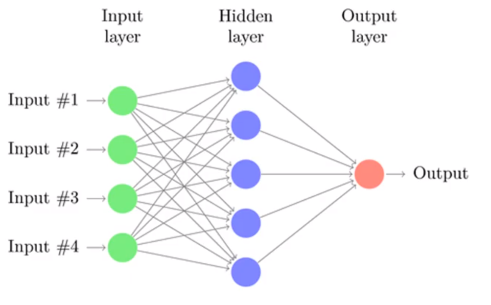
하지만 이 Multi Layer Perceptron을 학습시키는 방법을 몰랐다. 이는 후에 Backpropagation을 통해 학습시키게 된다.

Backpropagation

Backpropagation은 chain rule을 이용해 간단하게 Multi Layer Perceptron을 학습시킨다.

실제 코드를 통해 Backpropagtion을 통한 학습을 구현해본다.

import torch

torch.manual_seed(1)

device = 'cpu'

X = torch.FloatTensor([[0, 0], [0, 1], [1, 0], [1, 1]])
Y = torch.FloatTensor([[0], [1], [1], [0]])

# nn Layers
w1 = torch.Tensor(2, 2).to(device)
b1 = torch.Tensor(2).to(device)
w2 = torch.Tensor(2, 1).to(device)
b2 = torch.Tensor(1).to(device)

def sigmoid(x):
    return 1.0/(1.0+torch.exp(-x))

def sigmoid_prime(x):
    return sigmoid(x) * (1-sigmoid(x))

여기서 sigmoid_prime은 sigmoid를 미분한 함수이다. wieght와 bias 둘다 직접 선언한다.

learning_rate = 0.1
for step in range(10001):
    # forward
    l1 = torch.add(torch.matmul(X, w1), b1)
    a1 = sigmoid(l1)
    l2 = torch.add(torch.matmul(a1, w2), b2)
    Y_pred = sigmoid(l2)
    
    cost = -torch.mean(Y*torch.log(Y_pred)+(1-Y)*torch.log(1-Y_pred))
    
    # backprop with chain rule
    # cost
    d_Y_pred = (Y_pred-Y) / (Y_pred * (1.0 - Y_pred) + 1e-7)
    
    # Layer2
    d_l2 = d_Y_pred * sigmoid_prime(l2)
    d_b2 = d_l2
    d_w2 = torch.matmul(torch.transpose(a1, 0, 1), d_b2)
    
    # Layer1
    d_a1 = torch.matmul(d_b2, torch.transpose(w2, 0, 1))
    d_l1 = d_a1 * sigmoid_prime(l1)
    d_b1 = d_l1
    d_w1 = torch.matmul(torch.transpose(X, 0, 1), d_b1)
    
    #weight update
    w1 = w1 - learning_rate * d_w1
    b1 = b1 - learning_rate * torch.mean(d_b1, 0)
    w2 = w2 - learning_rate * d_w2
    b2 = b2 - learning_rate * torch.mean(d_b2, 0)
    
    if step%1000 == 0:
        print(step, cost.item())
'''
0 2.0181491374969482
1000 0.4068569242954254
2000 0.10715863853693008
3000 0.05720315873622894
4000 0.038493819534778595
5000 0.028874965384602547
6000 0.023054534569382668
7000 0.01916574127972126
8000 0.016388656571507454
9000 0.014308402314782143
10000 0.012693127617239952
'''

pytorch에서는 forward(), backward(), step() 으로 줄일 수 있다.

Code : xor-nn

지난 포스트에서는 linear 하나만 있었지만, MLP이므로 linear1, linear2를 만들어주고, Sequential에 추가해준다.

import torch

device = 'cpu'
torch.manual_seed(1)

X = torch.FloatTensor([[0, 0], [0, 1], [1, 0], [1, 1]]).to(device)
Y = torch.FloatTensor([[0], [1], [1], [0]]).to(device)

linear1 = torch.nn.Linear(2, 2, bias=True)
linear2 = torch.nn.Linear(2, 1, bias=True)
sigmoid = torch.nn.Sigmoid()
model = torch.nn.Sequential(linear1, sigmoid, linear2, sigmoid).to(device)

#define loss function and optimizer
criterion = torch.nn.BCELoss().to(device)
optimizer = torch.optim.SGD(model.parameters(), lr=1)

for step in range(10001):
    optimizer.zero_grad()
    hypothesis = model(X)
    
    cost = criterion(hypothesis, Y)
    cost.backward()
    
    optimizer.step()
    if step % 1000 == 0:
        print(step, cost.item())
'''
0 0.7027696967124939
1000 0.6191841959953308
2000 0.01236904039978981
3000 0.0053703682497143745
4000 0.0034116669557988644
5000 0.0024955791886895895
6000 0.0019656752701848745
7000 0.0016206535510718822
8000 0.0013782461173832417
9000 0.0011987212346866727
10000 0.0010604143608361483
'''

만들어진 모델을 평가해보면 정확도가 100%이다.

with torch.no_grad():
    hypothesis = model(X)
    predicted = (hypothesis > 0.5).float()
    accuracy = (predicted == Y).float().mean()
    print('\nHypothesis: ', hypothesis.detach().cpu().numpy(), '\nCorrect: ', predicted.detach().cpu().numpy(), '\nAccuracy: ', accuracy.item())
'''
Hypothesis:  [[0.00123878]
 [0.99904925]
 [0.99905175]
 [0.00110106]] 
Correct:  [[0.]
 [1.]
 [1.]
 [0.]] 
Accuracy:  1.0
'''

Code : xor-nn-wide-deep

네트워크가 깊어지고 넓어진다면 어떻게 될까.

기존 코드에서 층과 너비를 넓혀본다.

linear1 = torch.nn.Linear(2, 10, bias=True)
linear2 = torch.nn.Linear(10, 10, bias=True)
linear3 = torch.nn.Linear(10, 10, bias=True)
linear4 = torch.nn.Linear(10, 1, bias=True)
sigmoid = torch.nn.Sigmoid()
model = torch.nn.Sequential(linear1, sigmoid, linear2, sigmoid, linear3, sigmoid, linear4, sigmoid).to(device)
'''
0 0.7319304943084717
1000 0.6931300759315491
2000 0.6931138038635254
3000 0.6930681467056274
4000 0.6928067207336426
5000 0.5227216482162476
6000 0.0009290832094848156
7000 0.00041086674900725484
8000 0.0002585246111266315
9000 0.0001869827538030222
10000 0.00014578891568817198
'''

층이 깊고, 넓을 수록 loss가 점점 더 줄어드는 것을 확인할 수 있다.