다음 사이트를 참고하여 작성하였습니다.
https://seaborn.pydata.org/tutorial/introduction.html
파이썬의 대표적인 시각화 도구인 seaborn에 대해 정리해보려고 한다.
1. seaborn 소개
Seaborn은 Python에서 통계 그래픽을 만들기 위한 라이브러리이다. matplotlib 위에 구축되며 pandas 데이터구조와 밀접하게 통합된다.
시각화 하기 위한 단계를 간단하게 알아보자.
1) 다음과 같이 sns라는 약어로 seaborn을 불러온다.
# Import seaborn
import seaborn as sns
2) 기본 테마를 설정해준다.
# Apply the default theme
sns.set_theme()
3) tips라는 예시 데이터셋을 로드해준다.
load_dataset()함수를 사용하여 seaborn의 예제 데이터 세트에 빠르게 액세스 할 수 있다.
물론 pd.read_csv로 직접 로드할 수 있다.
tips = sns.load_dataset("tips")4) 시각화를 한다.
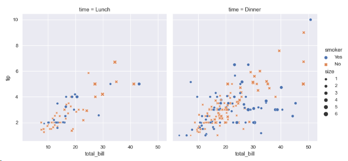
다음은 tips 데이터 세트의 5개 변수 간의 관계를 보여주는 코드이다. matplotlib를 직접 사용할 때와 달리 색상 값이나 마커에서 plot의 속성을 지정할 필요가 없다.
sns.relplot(
    data=tips,
    x="total_bill", y="tip", col="time",
    hue="smoker", style="smoker", size="size",
)
2. 통계를 위한 플롯
relplot()
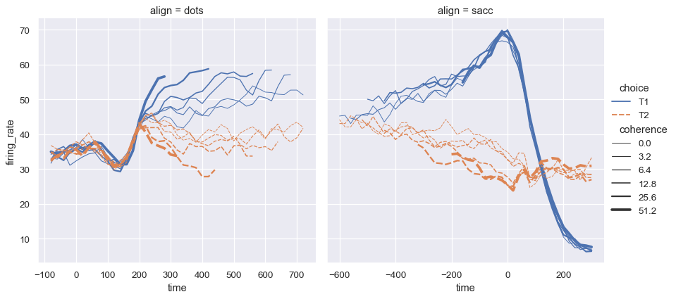
relplot은 다양한 통계적 관계를 시각화하도록 설계되었다. 보통 산점도가 효과적인 경우가 많지만 변수 중 시간을 나타내는 변수가 있을 경우에는 선으로 더 잘 표현된다. kind 변수를 사용하여 그래프 유형을 변경할 수 있다.
dots = sns.load_dataset("dots")
sns.relplot(
    data=dots, kind="line",
    x="time", y="firing_rate", col="align",
    hue="choice", size="coherence", style="choice",
    facet_kws=dict(sharex=False),
)
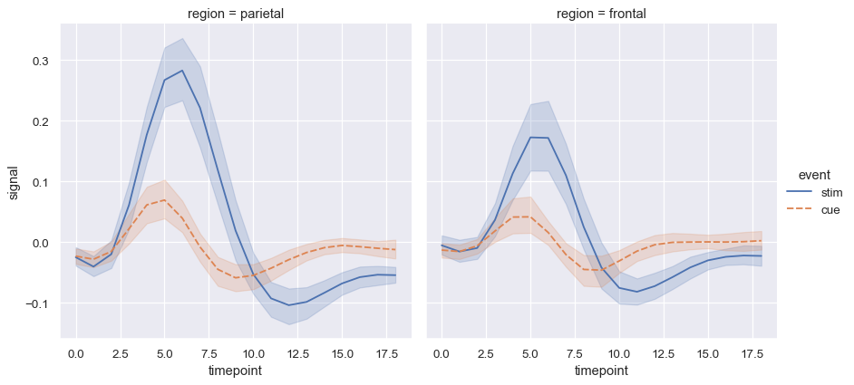
fmri = sns.load_dataset("fmri")
sns.relplot(
    data=fmri, kind="line",
    x="timepoint", y="signal", col="region",
    hue="event", style="event",
)
lmplot()
lmplot은 데이터의 산점도와 회귀선, 신뢰 구간을 함께 그려준다. 통계적으로 아주 유용하다.
sns.lmplot(data=tips, x="total_bill", y="tip", col="time", hue="smoker")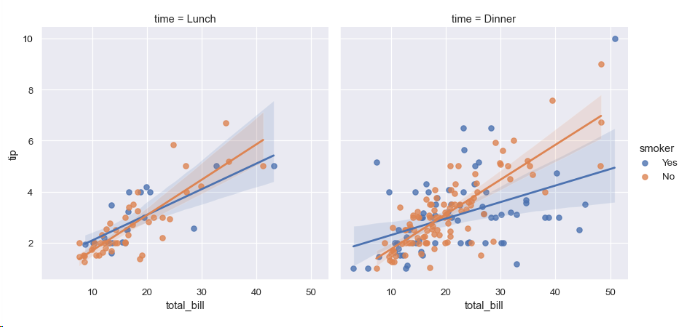
displot()
displot은 데이터의 분포를 시각화 하는데 도움을 준다. 여기에는 히스토그램, 커널 밀도 추정과 같은 방식이 포함된다.
sns.displot(data=tips, x="total_bill", col="time", kde=True)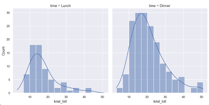
또한, 데이터의 누적 분포를 계산할 수도 있다.
sns.displot(data=tips, kind="ecdf", x="total_bill", col="time", hue="smoker", rug=True)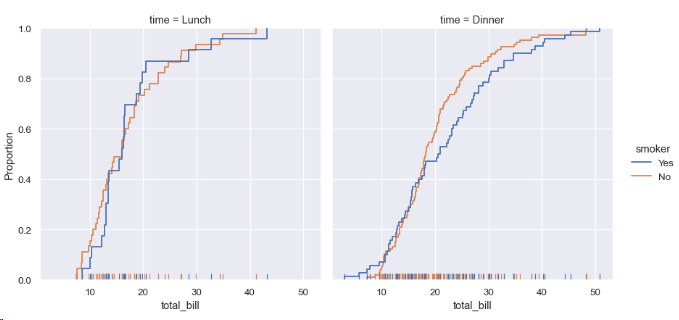
3. 범주형 데이터에 대한 플롯
catplot()
catplot은 가장 좋은 수준에서 군집 플롯을 그려 모든 관측값을 볼 수 있다. kind 변수로 다양한 시각화가 가능하다.
[swarm]
sns.catplot(data=tips, kind="swarm", x="day", y="total_bill", hue="smoker")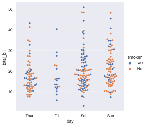
[violin]
sns.catplot(data=tips, kind="violin", x="day", y="total_bill", hue="smoker", split=True)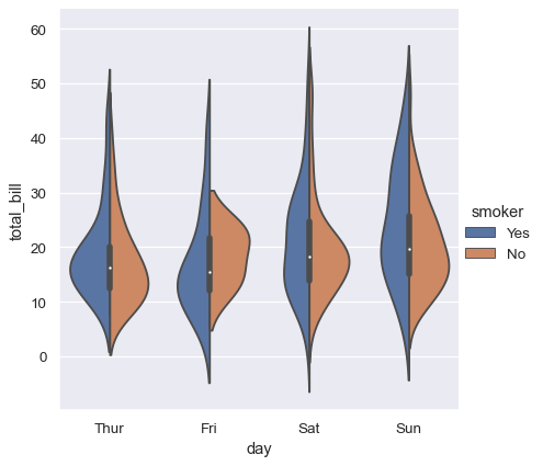
[bar]
또한, 각 범주 내에서 평균값과 신뢰 구간을 표시할 수도 있다.
sns.catplot(data=tips, kind="bar", x="day", y="total_bill", hue="smoker")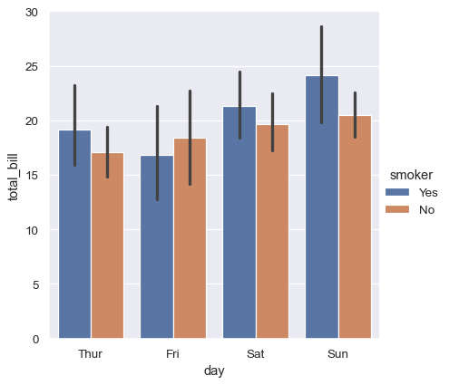
4. 복잡한 데이터 세트에 대한 다변량 보기
jointplot()
jointplot은 단일 관계에 중점을 둔다. 각 변수의 주변 분포와 함께 두 변수 간의 결합 분포를 시각화해준다.
penguins = sns.load_dataset("penguins")
sns.jointplot(data=penguins, x="flipper_length_mm", y="bill_length_mm", hue="species")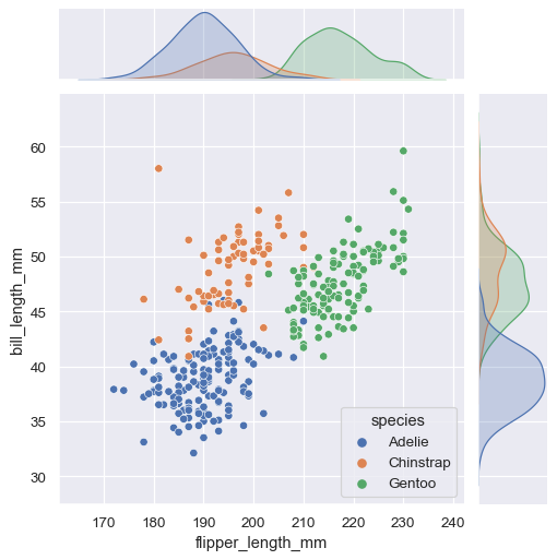
pairplot()
pairplot은 모든 데이터의 관계와 각 변수에 대한 분포를 각각 보여준다.
sns.pairplot(data=penguins, hue="species")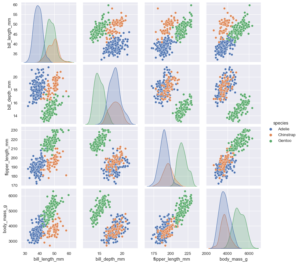
5. PairGrid
g = sns.PairGrid(penguins, hue="species", corner=True)
g.map_lower(sns.kdeplot, hue=None, levels=5, color=".2")
g.map_lower(sns.scatterplot, marker="+")
g.map_diag(sns.histplot, element="step", linewidth=0, kde=True)
g.add_legend(frameon=True)
g.legend.set_bbox_to_anchor((.61, .6))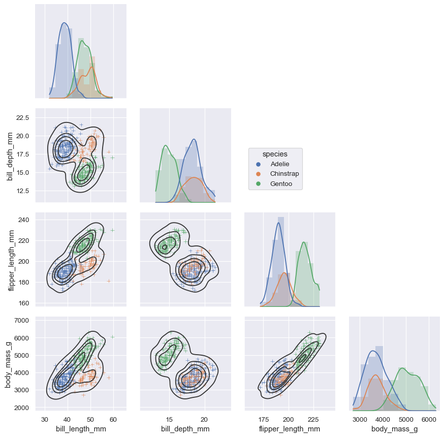
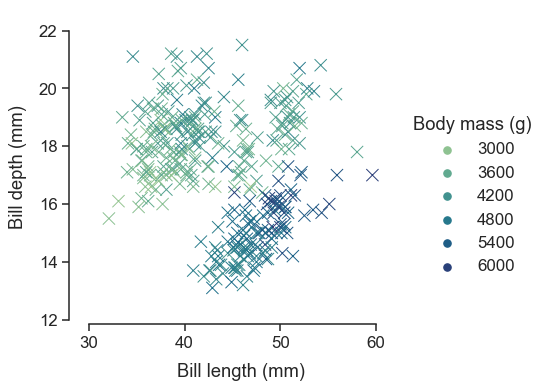
6. 사용자 정의
seaborn은 다음과 같이 사용자가 다양하게 정의하여 그래프를 다듬을 수 있다.
sns.set_theme(style="ticks", font_scale=1.25)
g = sns.relplot(
    data=penguins,
    x="bill_length_mm", y="bill_depth_mm", hue="body_mass_g",
    palette="crest", marker="x", s=100,
)
g.set_axis_labels("Bill length (mm)", "Bill depth (mm)", labelpad=10)
g.legend.set_title("Body mass (g)")
g.figure.set_size_inches(6.5, 4.5)
g.ax.margins(.15)
g.despine(trim=True)