- 서베이 데이터를 이용해 하나의 스토리를 만들어내는 컴피티션이지만 EDA 연습용으로 사용해보자.
- pandas나 matplotlib는 힘들게 배워놔도 이렇게 계속 써주지 않으면 까먹는다..
- 퓨쳐스킬 과제로 진행
# This Python 3 environment comes with many helpful analytics libraries installed
# It is defined by the kaggle/python Docker image: https://github.com/kaggle/docker-python
# For example, here's several helpful packages to load

import numpy as np # linear algebra
import pandas as pd # data processing, CSV file I/O (e.g. pd.read_csv)
import matplotlib.pyplot as plt
import seaborn as sns
df = pd.read_csv('/kaggle/input/kaggle-survey-2020/kaggle_survey_2020_responses.csv')# 어떤 질문들이 있는지 확인
for col, question in zip(df.columns, df.iloc[0]):
print(f'{col} ::: {question}')궁금한 내용
- 주로 사용하는 언어
- 직무별 배우고싶은 categories of automated machine learning tools
- 직무별로 ML직접 사용비율/tool 사용비율이 다를까?
설문자 나이/성별/직무 분포
age_x = df.iloc[1:].groupby(by='Q1')['Q1'].count().index
age_y = df.iloc[1:].groupby(by='Q1')['Q1'].count().values
gender_x = df.iloc[1:].groupby(by='Q2')['Q2'].count().index
gender_y = df.iloc[1:].groupby(by='Q2')['Q2'].count().valuesrole_x = df.iloc[1:].groupby(by='Q5')['Q5'].count().index
role_y = df.iloc[1:].groupby(by='Q5')['Q5'].count().valuesfig, (ax_age, ax_gender) = plt.subplots(1, 2, figsize=(20, 4))
ax_age.bar(age_x, age_y)
ax_age.set_title('age count')
ax_gender.bar(gender_x, gender_y)
ax_gender.set_title('gender count')
plt.show()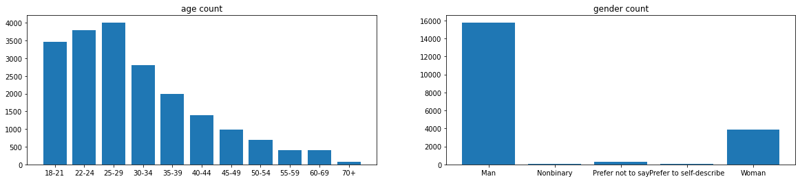
fig, ax_role = plt.subplots(figsize=(10, 4))

colors = sns.color_palette('hls', len(role_x))
bars = ax_role.bar(role_x, role_y, color=colors)
ax_role.set_title('role count')
ax_role.legend(bars, role_x, loc='upper left', bbox_to_anchor=(1, 1))
ax_role.get_xaxis().set_visible(False)

plt.show()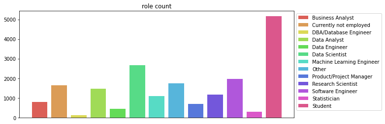
- xticks label이 긴 경우 그냥 legend로 빼버리는게 나은것같다.
- 학생이 압도적으로 많다..
- 학생을 제외하면 데싸-소프트웨어 엔지니어-기타등등
주 사용 언어
df.loc[:, 'Q7_Part_1':'Q7_OTHER']| Q7_Part_1 | Q7_Part_2 | Q7_Part_3 | Q7_Part_4 | Q7_Part_5 | Q7_Part_6 | Q7_Part_7 | Q7_Part_8 | Q7_Part_9 | Q7_Part_10 | Q7_Part_11 | Q7_Part_12 | Q7_OTHER | |
|---|---|---|---|---|---|---|---|---|---|---|---|---|---|
| 0 | What programming languages do you use on a reg... | What programming languages do you use on a reg... | What programming languages do you use on a reg... | What programming languages do you use on a reg... | What programming languages do you use on a reg... | What programming languages do you use on a reg... | What programming languages do you use on a reg... | What programming languages do you use on a reg... | What programming languages do you use on a reg... | What programming languages do you use on a reg... | What programming languages do you use on a reg... | What programming languages do you use on a reg... | What programming languages do you use on a reg... |
| 1 | Python | R | SQL | C | NaN | NaN | Javascript | NaN | NaN | NaN | MATLAB | NaN | Other |
| 2 | Python | R | SQL | NaN | NaN | NaN | NaN | NaN | NaN | NaN | NaN | NaN | NaN |
| 3 | NaN | NaN | NaN | NaN | NaN | Java | Javascript | NaN | NaN | Bash | NaN | NaN | NaN |
| 4 | Python | NaN | SQL | NaN | NaN | NaN | NaN | NaN | NaN | Bash | NaN | NaN | NaN |
| ... | ... | ... | ... | ... | ... | ... | ... | ... | ... | ... | ... | ... | ... |
| 20032 | NaN | NaN | NaN | NaN | NaN | NaN | NaN | NaN | NaN | NaN | NaN | NaN | NaN |
| 20033 | Python | NaN | NaN | NaN | NaN | NaN | NaN | NaN | NaN | NaN | NaN | NaN | NaN |
| 20034 | Python | NaN | NaN | NaN | NaN | NaN | NaN | NaN | NaN | NaN | NaN | NaN | NaN |
| 20035 | Python | NaN | SQL | C | NaN | Java | Javascript | NaN | NaN | NaN | NaN | NaN | NaN |
| 20036 | Python | NaN | NaN | NaN | NaN | NaN | NaN | NaN | NaN | NaN | NaN | NaN | NaN |
20037 rows × 13 columns
- 다중선택 질문의 경우 각 선택지마다 column이 있고, 해당 항목을 선택하지 않은 경우 None이 수집된다.
- 이 df에 count를 해주면 None이 아닌 값만 count된다.
lang_x = ['Python','R','SQL','C','C++','Java','Javascript','Julia','Swift','Bash','MATLAB','None','Other']
lang_y = df.loc[:, 'Q7_Part_1':'Q7_OTHER'].count()

fig, ax_lang = plt.subplots(figsize=(10, 4))

ax_lang.bar(lang_x, lang_y)
ax_lang.set_title('lang count')

plt.show()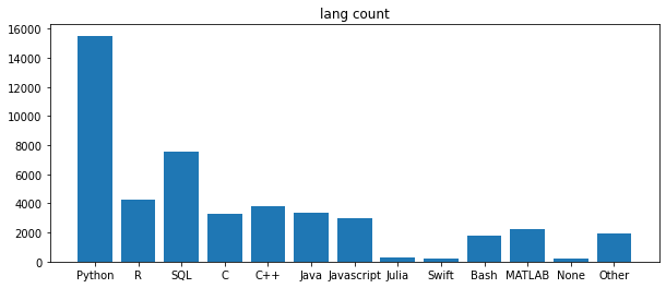
- 예상대로 python이 압도적, 캐글 설문답게 SQL도 우세
- 직무별 추천하는 언어가 다를까?
df.iloc[1:].groupby(['Q5', 'Q8'])['Q8'].count()Q5 Q8
Business Analyst C 9
C++ 5
Java 4
Javascript 6
Julia 3
...
Student Other 28
Python 3921
R 273
SQL 89
Swift 4
Name: Q8, Length: 155, dtype: int64- 직무별, 언어별로 일단 count를 해본다.
- multi index로 들어가있는 언어를 column으로 돌리기 위해 unstack을 해준다.
df.iloc[1:].groupby(['Q5', 'Q8'])['Q8'].count().unstack()| Q8 | Bash | C | C++ | Java | Javascript | Julia | MATLAB | None | Other | Python | R | SQL | Swift |
|---|---|---|---|---|---|---|---|---|---|---|---|---|---|
| Q5 | |||||||||||||
| Business Analyst | NaN | 9.0 | 5.0 | 4.0 | 6.0 | 3.0 | 3.0 | 1.0 | 9.0 | 501.0 | 77.0 | 63.0 | 4.0 |
| Currently not employed | 3.0 | 14.0 | 15.0 | 16.0 | 7.0 | 3.0 | 11.0 | 7.0 | 11.0 | 1220.0 | 84.0 | 67.0 | 2.0 |
| DBA/Database Engineer | NaN | 2.0 | 1.0 | 2.0 | 1.0 | 1.0 | NaN | 1.0 | 2.0 | 92.0 | 6.0 | 13.0 | NaN |
| Data Analyst | 3.0 | 13.0 | 13.0 | 8.0 | 13.0 | 4.0 | 10.0 | 5.0 | 4.0 | 977.0 | 136.0 | 167.0 | NaN |
| Data Engineer | 1.0 | 6.0 | 7.0 | 3.0 | 3.0 | 2.0 | 3.0 | 1.0 | 7.0 | 336.0 | 15.0 | 33.0 | 1.0 |
| Data Scientist | 3.0 | 17.0 | 20.0 | 14.0 | 6.0 | 20.0 | 13.0 | 3.0 | 17.0 | 2087.0 | 217.0 | 187.0 | 2.0 |
| Machine Learning Engineer | 2.0 | 18.0 | 31.0 | 3.0 | 4.0 | 7.0 | 23.0 | NaN | 7.0 | 894.0 | 27.0 | 23.0 | NaN |
| Other | 2.0 | 16.0 | 18.0 | 9.0 | 5.0 | 15.0 | 12.0 | 14.0 | 21.0 | 1191.0 | 110.0 | 79.0 | NaN |
| Product/Project Manager | NaN | 5.0 | 11.0 | 9.0 | 2.0 | 3.0 | 5.0 | 10.0 | 12.0 | 464.0 | 40.0 | 40.0 | 1.0 |
| Research Scientist | 3.0 | 27.0 | 30.0 | 11.0 | 8.0 | 18.0 | 33.0 | 4.0 | 8.0 | 846.0 | 108.0 | 10.0 | NaN |
| Software Engineer | 4.0 | 40.0 | 36.0 | 35.0 | 18.0 | 12.0 | 19.0 | 5.0 | 18.0 | 1575.0 | 76.0 | 62.0 | 3.0 |
| Statistician | NaN | 4.0 | 8.0 | 1.0 | NaN | 1.0 | 1.0 | NaN | 7.0 | 137.0 | 90.0 | 16.0 | NaN |
| Student | 5.0 | 130.0 | 130.0 | 52.0 | 15.0 | 32.0 | 62.0 | 30.0 | 28.0 | 3921.0 | 273.0 | 89.0 | 4.0 |
- NaN값이 많고, 단순 카운트는 직무별 응답자 수 차이가 있어 값을 정규화해야 보기 좋을 것 같다.
- 각 값을 직무별 응답자 수에 대한 비율로 만들어주기 위해, 각 직무별 sum을 먼저 구한 후 그 값으로 나눠준다.
lang_by_role_df = df.iloc[1:].groupby(['Q5', 'Q8'])['Q8'].count().unstack()
per_lang_by_role = lang_by_role_df.div(lang_by_role_df.sum(axis=1), axis=0)per_lang_by_role| Q8 | Bash | C | C++ | Java | Javascript | Julia | MATLAB | None | Other | Python | R | SQL | Swift |
|---|---|---|---|---|---|---|---|---|---|---|---|---|---|
| Q5 | |||||||||||||
| Business Analyst | NaN | 0.013139 | 0.007299 | 0.005839 | 0.008759 | 0.004380 | 0.004380 | 0.001460 | 0.013139 | 0.731387 | 0.112409 | 0.091971 | 0.005839 |
| Currently not employed | 0.002055 | 0.009589 | 0.010274 | 0.010959 | 0.004795 | 0.002055 | 0.007534 | 0.004795 | 0.007534 | 0.835616 | 0.057534 | 0.045890 | 0.001370 |
| DBA/Database Engineer | NaN | 0.016529 | 0.008264 | 0.016529 | 0.008264 | 0.008264 | NaN | 0.008264 | 0.016529 | 0.760331 | 0.049587 | 0.107438 | NaN |
| Data Analyst | 0.002217 | 0.009608 | 0.009608 | 0.005913 | 0.009608 | 0.002956 | 0.007391 | 0.003695 | 0.002956 | 0.722099 | 0.100517 | 0.123429 | NaN |
| Data Engineer | 0.002392 | 0.014354 | 0.016746 | 0.007177 | 0.007177 | 0.004785 | 0.007177 | 0.002392 | 0.016746 | 0.803828 | 0.035885 | 0.078947 | 0.002392 |
| Data Scientist | 0.001151 | 0.006523 | 0.007675 | 0.005372 | 0.002302 | 0.007675 | 0.004988 | 0.001151 | 0.006523 | 0.800844 | 0.083269 | 0.071757 | 0.000767 |
| Machine Learning Engineer | 0.001925 | 0.017324 | 0.029836 | 0.002887 | 0.003850 | 0.006737 | 0.022137 | NaN | 0.006737 | 0.860443 | 0.025987 | 0.022137 | NaN |
| Other | 0.001340 | 0.010724 | 0.012064 | 0.006032 | 0.003351 | 0.010054 | 0.008043 | 0.009383 | 0.014075 | 0.798257 | 0.073727 | 0.052949 | NaN |
| Product/Project Manager | NaN | 0.008306 | 0.018272 | 0.014950 | 0.003322 | 0.004983 | 0.008306 | 0.016611 | 0.019934 | 0.770764 | 0.066445 | 0.066445 | 0.001661 |
| Research Scientist | 0.002712 | 0.024412 | 0.027125 | 0.009946 | 0.007233 | 0.016275 | 0.029837 | 0.003617 | 0.007233 | 0.764919 | 0.097649 | 0.009042 | NaN |
| Software Engineer | 0.002102 | 0.021019 | 0.018917 | 0.018392 | 0.009459 | 0.006306 | 0.009984 | 0.002627 | 0.009459 | 0.827641 | 0.039937 | 0.032580 | 0.001576 |
| Statistician | NaN | 0.015094 | 0.030189 | 0.003774 | NaN | 0.003774 | 0.003774 | NaN | 0.026415 | 0.516981 | 0.339623 | 0.060377 | NaN |
| Student | 0.001048 | 0.027248 | 0.027248 | 0.010899 | 0.003144 | 0.006707 | 0.012995 | 0.006288 | 0.005869 | 0.821840 | 0.057221 | 0.018654 | 0.000838 |
fig, ax_lang_role = plt.subplots(figsize=(10, 10))
ax_lang_role = sns.heatmap(per_lang_by_role, vmin=-0.1)
plt.title('language recommendation', fontsize=20)
plt.show() 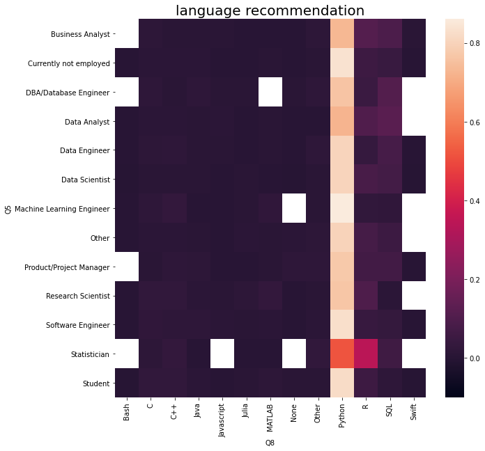
- 파이썬이 압도적
- 상대적으로 Business analyst, Data analyst, Data scientist, Research scientist가 다른 직무에 비해 R을 추천하는 경향
Tool 관련
tool_x = ['data augmentation','feature engineering','model selection','model architecture searches','hyperparameter tuning','full ML pipelines','None','Other']
tool_y = df.loc[:, 'Q33_B_Part_1':'Q33_B_OTHER'].count()

fig, ax_tool = plt.subplots(figsize=(5, 5))

colors = sns.color_palette('hls', len(tool_x))
bars = ax_tool.bar(tool_x, tool_y, color=colors)
ax_tool.set_title('tool count')
ax_tool.legend(bars, tool_x, loc='upper left', bbox_to_anchor=(1, 1))
ax_tool.get_xaxis().set_visible(False)

plt.show()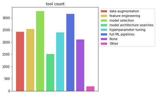
- 전반적으로 관심이 높지만 model selection, pipeline에 관심도가 높다
# 각 분야의 직무별 비율
df_tool_and_role = df.loc[1:, ['Q5', 'Q33_B_Part_1', 'Q33_B_Part_2', 'Q33_B_Part_3', 'Q33_B_Part_4', 'Q33_B_Part_5', 'Q33_B_Part_6', 'Q33_B_Part_7', 'Q33_B_OTHER']].groupby('Q5').count()
df_tool_and_role = df_tool_and_role.swapaxes(0, 1)
df_tool_and_role.index = tool_x
colors = sns.color_palette('hls', len(df_tool_and_role.columns))
df_tool_and_role.plot.bar(stacked=True, figsize=(10, 10), color=colors)<AxesSubplot:>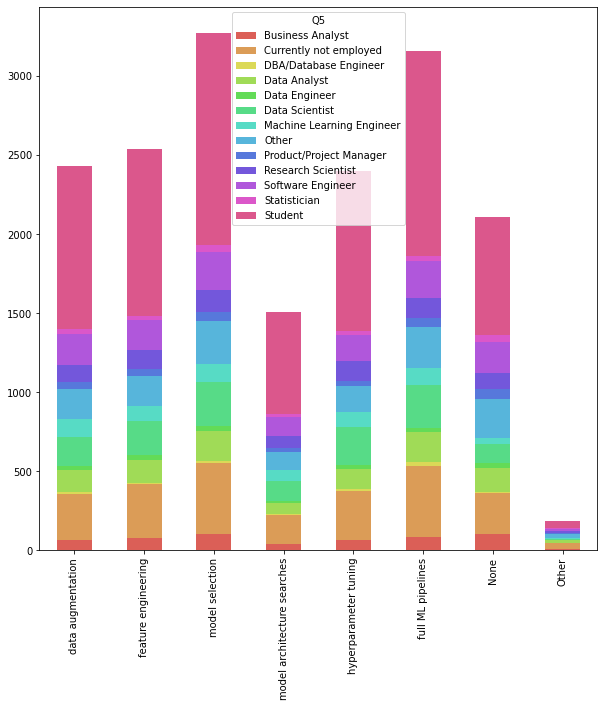
- 직군 수에 차이가 있어 눈에 띄지 않는다. 비율로 바꿔보자
- not employed와 Other, student와 수가 적은 statistician, DBA는 빼보자
per_df_tool_and_role = df_tool_and_role.div(df_tool_and_role.sum(axis=0), axis=1)
per_df_tool_and_role = per_df_tool_and_role.iloc[:, [0, 3, 4, 5, 6, 8, 9, 10]]
colors = sns.color_palette('hls', len(per_df_tool_and_role.columns))
per_df_tool_and_role.plot.bar(stacked=True, figsize=(10, 10), color=colors)<AxesSubplot:>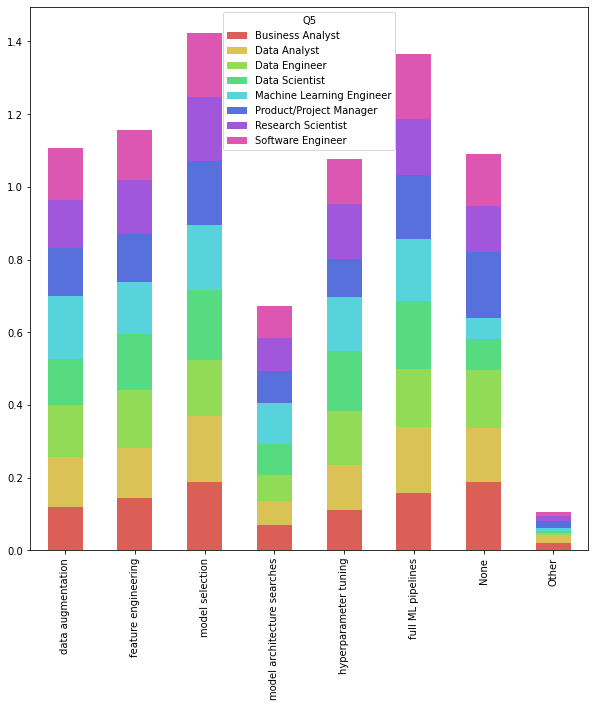
- 줄무늬 도마뱀같다.
- 대부분 고른 분포.. 별 차이는 없었다
- 뭘 배우고 싶지 않은 PM들이 많다.
- ml 엔지니어들이 다른 직무에 비해 data augmentation이나 model architecture search를 배우고 싶어하고, None으로 응답한 비율이 가장 적다. 학구열이 가장 높은 집단 아닐까? 생존을 위해 배워야 한다거나
# 자연어처리 모델은 뭘 쓰는지도 궁금하다
models_x = ['Word embeddings/vectors', 'Encoder-decorder models', 'Contextualized embeddings', 'Transformer language models', 'None', 'Other']
models_y = df[1:].loc[:, 'Q19_Part_1':'Q19_OTHER'].count().values

fig, ax = plt.subplots(figsize=(5, 5))
colors = sns.color_palette('hls', len(models_x))
bars = ax.bar(models_x, models_y, color=colors)
ax.legend(bars, models_x, loc='upper left', bbox_to_anchor=(1, 1))
ax.get_xaxis().set_visible(False)
plt.show()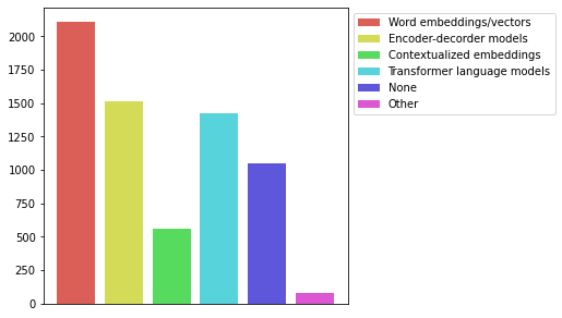
- 아직은 word embedding도 죽지 않았다.. 가성비도 중요한것같다

developer hamdoe