네이버 영화리뷰 데이터를 가지고 감성을 분석합니다.
[https://github.com/e9t/nsmc]
데이터 호출
- 데이터를 train과 test에 저장하겠습니다
import pandas as pd
import urllib.request
%matplotlib inline
import matplotlib.pyplot as plt
import re
from konlpy.tag import Okt
from tensorflow import keras
from tensorflow.keras.preprocessing.text import Tokenizer
import numpy as np
from tensorflow.keras.preprocessing.sequence import pad_sequences
from collections import Counter

# 데이터를 읽어봅시다.
train_data = pd.read_table('~/aiffel/sentiment_classification/data/ratings_train.txt')
test_data = pd.read_table('~/aiffel/sentiment_classification/data/ratings_test.txt')

train_data.head()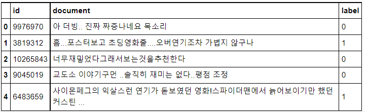
데이터 전처리
- 위에서 확인한 것처럼 데이터의 전처리가 필요해 보입니다.
- 데이터 중복을 제거
- 결측치 제거
- 한국어 토크나이저로 토큰화
- 불용어 제거
- 사전 word_to_index 구성
- 텍스트 스트링을 사전 인덱스 스트링으로 변환
- X_train, y_train, X_test, y_test 리턴
from konlpy.tag import Mecab
tokenizer = Mecab()
stopwords = ['의','가','이','은','들','는','좀','잘','걍','과','도','를','으로','자','에','와','한','하다']

def load_data(train_data, test_data, num_words=10000):
    #데이터의 중복을 제거
    train_data.drop_duplicates(subset=['document'], inplace=True)
    #데이터의 결측치를 제거
    train_data = train_data.dropna(how = 'any')
    test_data.drop_duplicates(subset=['document'], inplace=True)
    test_data = test_data.dropna(how = 'any')

    X_train = []
    for sentence in train_data['document']:
        #데이터를 토큰화 시킨다 ex) 안녕 = 1
        temp_X = tokenizer.morphs(sentence) # 토큰화
        #stopwords에 있는 불용어들이 문장에 있으면 제거 해줍니다.
        temp_X = [word for word in temp_X if not word in stopwords] # 불용어 제거
        X_train.append(temp_X)

    X_test = []
    for sentence in test_data['document']:
        temp_X = tokenizer.morphs(sentence) # 토큰화
        temp_X = [word for word in temp_X if not word in stopwords] # 불용어 제거
        X_test.append(temp_X)

    words = np.concatenate(X_train).tolist()
    counter = Counter(words)
    counter = counter.most_common(10000-4)
    vocab = ['', '', '', ''] + [key for key, _ in counter]
    word_to_index = {word:index for index, word in enumerate(vocab)}

    def wordlist_to_indexlist(wordlist):
        return [word_to_index[word] if word in word_to_index else word_to_index[''] for word in wordlist]

    X_train = list(map(wordlist_to_indexlist, X_train))
    X_test = list(map(wordlist_to_indexlist, X_test))

    return X_train, np.array(list(train_data['label'])), X_test, np.array(list(test_data['label'])), word_to_index

X_train, y_train, X_test, y_test, word_to_index = load_data(train_data, test_data)
문장의 길의 확인
- 나중 전처리에 포함될 예정이지만 문장의 길이를 확인하는 이유는 나중에 문장길이를 동일하게 맞출 필요가 있습니다. 토큰화 된 문장들에 빈자리는 0으로 채우는 것이지요!
print(X_train[0])  # 1번째 리뷰데이터
print('라벨: ', y_train[0])  # 1번째 리뷰데이터의 라벨
print('1번째 리뷰 문장 길이: ', len(X_train[0]))
print('2번째 리뷰 문장 길이: ', len(X_train[1]))
[32, 74, 919, 4, 4, 39, 228, 20, 33, 748]
라벨: 0
1번째 리뷰 문장 길이: 10
2번째 리뷰 문장 길이: 17
index to word와 word to index 딕셔너리를 생성합니다.
단어들이 어떤식으로 토큰화가 되어있는지 확인하기 편리합니다. 숫자를 문자로, 문자를 숫자로 확인하기 편리해 지는 것이지용!
index_to_word = {index:word for word, index in word_to_index.items()}# 문장 1개를 활용할 딕셔너리와 함께 주면, 단어 인덱스 리스트 벡터로 변환해 주는 함수입니다.
# 단, 모든 문장은 <BOS>로 시작하는 것으로 합니다.
def get_encoded_sentence(sentence, word_to_index):
return [word_to_index['<BOS>']]+[word_to_index[word] if word in word_to_index else word_to_index['<UNK>'] for word in sentence.split()]
# 여러 개의 문장 리스트를 한꺼번에 단어 인덱스 리스트 벡터로 encode해 주는 함수입니다.
def get_encoded_sentences(sentences, word_to_index):
return [get_encoded_sentence(sentence, word_to_index) for sentence in sentences]
# 숫자 벡터로 encode된 문장을 원래대로 decode하는 함수입니다.
def get_decoded_sentence(encoded_sentence, index_to_word):
return ' '.join(index_to_word[index] if index in index_to_word else '<UNK>' for index in encoded_sentence[1:]) #[1:]를 통해 <BOS>를 제외
# 여러 개의 숫자 벡터로 encode된 문장을 한꺼번에 원래대로 decode하는 함수입니다.
def get_decoded_sentences(encoded_sentences, index_to_word):
return [get_decoded_sentence(encoded_sentence, index_to_word) for encoded_sentence in encoded_sentences]토큰화해서 저장한 Train 데이터들을 decode해서 확인해보겠습니다.
- 위에서 확인했듯 X_train은 토큰화된 숫자로 이뤄져있습니다. decode해주는 함수를 통해 문장을 확인할 수 있습니다.
decoded_sentences = get_decoded_sentences(X_train, index_to_word)print(decoded_sentences[0:5])['더 빙 . . 진짜 짜증 나 네요 목소리', '. .. 포스터 보고 초딩 영화 줄 . ... 오버 연기 조차 가볍 지 않 구나', '재 ', '이야기 구먼 . . 솔직히 재미 없 다 . . 평점 조정', '익살 스런 연기 돋보였 던 영화 ! 스파이더맨 에서 늙 어 보이 기 만 했 던 너무나 이뻐 보였 다']
PAD, BOS, UNK, UNUSED 를 추가하는 작업을 합니다.
- 문장의 길이를 맞추면 부족한 부분은 0으로 채워지기 때문입니다.
#실제 인코딩 인덱스는 제공된 word_to_index에서 index 기준으로 3씩 뒤로 밀려 있습니다.
word_to_index = {k:(v+1) for k,v in word_to_index.items()}

# 처음 몇 개 인덱스는 사전에 정의되어 있습니다
word_to_index["<PAD>"] = 0
word_to_index["<BOS>"] = 1
word_to_index["<UNK>"] = 2  # unknown
word_to_index["<UNUSED>"] = 3

index_to_word[0] = "<PAD>"
index_to_word[1] = "<BOS>"
index_to_word[2] = "<UNK>"
index_to_word[3] = "<UNUSED>"

index_to_word = {index:word for word, index in word_to_index.items()}

print(index_to_word[1]) # '<BOS>' 가 출력됩니다.total_data_text = list(X_train) + list(X_test)
# 텍스트데이터 문장길이의 리스트를 생성한 후
num_tokens = [len(tokens) for tokens in total_data_text]
num_tokens = np.array(num_tokens)
# 문장길이의 평균값, 최대값, 표준편차를 계산해 본다.
print('문장길이 평균 : ', np.mean(num_tokens))
print('문장길이 최대 : ', np.max(num_tokens))
print('문장길이 표준편차 : ', np.std(num_tokens))
# 예를들어, 최대 길이를 (평균 + 2*표준편차)로 한다면,
max_tokens = np.mean(num_tokens) + 2 * np.std(num_tokens)
maxlen = int(max_tokens)
print('pad_sequences maxlen : ', maxlen)
print('전체 문장의 {}%가 maxlen 설정값 이내에 포함됩니다. '.format(np.sum(num_tokens < max_tokens) / len(num_tokens)))문장길이 평균 : 15.96940191154864
문장길이 최대 : 116
문장길이 표준편차 : 12.843571191092
pad_sequences maxlen : 41
전체 문장의 0.9342988343341575%가 maxlen 설정값 이내에 포함됩니다.
문장에 앞에 0을 채워 넣는것이 더 좋은 분석이 된다고 해서 앞에 0을 채웁니다.
- 그 이유는 RNN 특성상 분석을 하다가 마지막에 답을 호출하기 때문입니다. 문장을 맞추기 위해 뒤에 0을 채우면 문장마다 다 0으로 끝나버리기 때문에 RNN이 조금 이상하겠죠,,,?
X_train = keras.preprocessing.sequence.pad_sequences(X_train,
                                                        value=word_to_index["<PAD>"],
                                                        padding='pre', # 혹은 'pre'
                                                        maxlen=maxlen)

X_test = keras.preprocessing.sequence.pad_sequences(X_test,
                                                       value=word_to_index["<PAD>"],
                                                       padding='pre', # 혹은 'pre'
                                                       maxlen=maxlen)

print(X_train.shape)
X_train[0]
(146182, 41)
Out[105]:
array([ 0, 0, 0, 0, 0, 0, 0, 0, 0, 0, 0, 0, 0,
0, 0, 0, 0, 0, 0, 0, 0, 0, 0, 0, 0, 0,
0, 0, 0, 0, 0, 32, 74, 919, 4, 4, 39, 228, 20,
33, 748], dtype=int32)
train의 일부를 validation으로 나누자
- train, validation을 80:20으로 나누겠습니다
from sklearn.model_selection import train_test_split
X_train, X_val, y_train, y_val = train_test_split(X_train,
                                                          y_train,
                                                          test_size=0.2,
                                                          shuffle=True,
                                                          random_state=34)
LSTM모델에 넣어 분석해보자
vocab_size = 10000    # 어휘 사전의 크기입니다(10,000개의 단어)
word_vector_dim = 41  # 워드 벡터의 차원 수 (변경 가능한 하이퍼파라미터)

# model 설계 - 딥러닝 모델 코드를 직접 작성해 주세요.
model = keras.Sequential()
model.add(keras.layers.Embedding(vocab_size, word_vector_dim, input_shape=(None,)))
model.add(keras.layers.LSTM(512))   # 가장 널리 쓰이는 RNN인 LSTM 레이어를 사용하였습니다. 이때 LSTM state 벡터의 차원수는 8로 하였습니다. (변경 가능)
model.add(keras.layers.Dense(8, activation='relu'))
model.add(keras.layers.Dense(1, activation='sigmoid'))  # 최종 출력은 긍정/부정을 나타내는 1dim 입니다.

model.summary()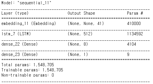
model.compile(optimizer='adam',
              loss='binary_crossentropy',
              metrics=['accuracy'])
earlystopping을 이용해서 과적합을 방지합니다!
from keras.callbacks import EarlyStopping
es=EarlyStopping(monitor='val_loss',mode='min',verbose=1,patience=10)
history = model.fit(X_train,
y_train,
epochs=20,
batch_size=512,callbacks=[es],
validation_data=(X_val, y_val),
verbose=1)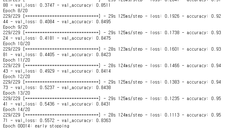
결과를 보니 85%에는 아직 모자릅니다
results = model.evaluate(X_test,  y_test, verbose=2)

print(results)
1537/1537 - 12s - loss: 0.5411 - accuracy: 0.8364
[0.5410551428794861, 0.8363610506057739]
LSTM모델 그래프로 그려보기
history_dict = history.history
print(history_dict.keys())
import matplotlib.pyplot as plt
acc = history_dict['accuracy']
val_acc = history_dict['val_accuracy']
loss = history_dict['loss']
val_loss = history_dict['val_loss']
epochs = range(1, len(acc) + 1)
# "bo"는 "파란색 점"입니다
plt.plot(epochs, loss, 'bo', label='Training loss')
# b는 "파란 실선"입니다
plt.plot(epochs, val_loss, 'b', label='Validation loss')
plt.title('Training and validation loss')
plt.xlabel('Epochs')
plt.ylabel('Loss')
plt.legend()
plt.show()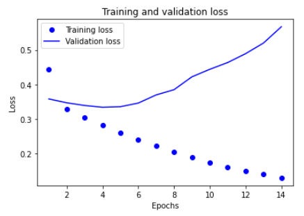
그래프를 보니 Training의 loss는 점점 줄었지만 validation은 늘었습니다. 과적합이 되면서 점점 못맞추게 되는 걸까요,,?
plt.clf() # 그림을 초기화합니다
plt.plot(epochs, acc, 'bo', label='Training acc')
plt.plot(epochs, val_acc, 'b', label='Validation acc')
plt.title('Training and validation accuracy')
plt.xlabel('Epochs')
plt.ylabel('Accuracy')
plt.legend()
plt.show()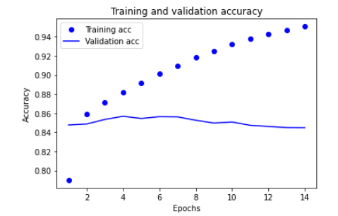
정확도도 train은 점점 잘 맞추는 반면 validation은 고만고만 합니다!
1-D CNN 적용하기
model = keras.Sequential()
model.add(keras.layers.Embedding(vocab_size, word_vector_dim, input_shape=(None,)))
model.add(keras.layers.Conv1D(16, 7, activation='relu'))
model.add(keras.layers.MaxPooling1D(5))
model.add(keras.layers.Conv1D(16, 7, activation='relu'))
model.add(keras.layers.GlobalMaxPooling1D())
model.add(keras.layers.Dense(8, activation='relu'))
model.add(keras.layers.Dense(1, activation='sigmoid')) # 최종 출력은 긍정/부정을 나타내는 1dim 입니다.
model.summary()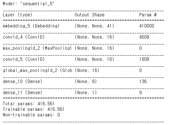
model.compile(optimizer='adam',
loss='binary_crossentropy',
metrics=['accuracy'])history = model.fit(X_train,
y_train,
epochs=20,
batch_size=512,callbacks=[es],
validation_data=(X_val, y_val),
verbose=1)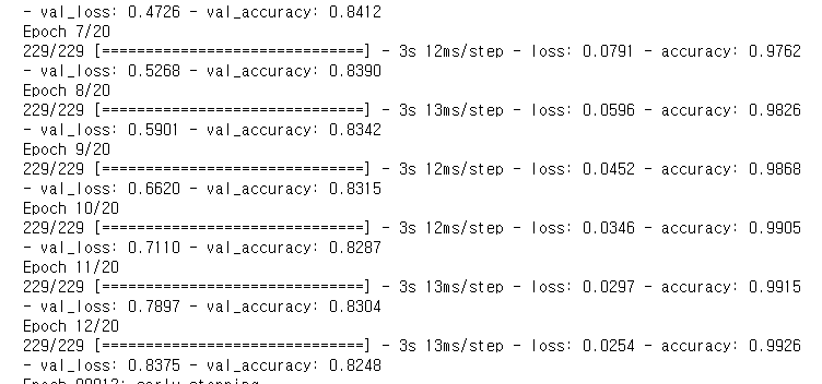
results = model.evaluate(X_test, y_test, verbose=2)
print(results)1537/1537 - 4s - loss: 0.8336 - accuracy: 0.8227
[0.8335745930671692, 0.8227109313011169]
1-D CNN 그래프로 그려보기
history_dict = history.history
print(history_dict.keys())dict_keys(['loss', 'accuracy', 'val_loss', 'val_accuracy'])
import matplotlib.pyplot as plt

acc = history_dict['accuracy']
val_acc = history_dict['val_accuracy']
loss = history_dict['loss']
val_loss = history_dict['val_loss']

epochs = range(1, len(acc) + 1)

# "bo"는 "파란색 점"입니다
plt.plot(epochs, loss, 'bo', label='Training loss')
# b는 "파란 실선"입니다
plt.plot(epochs, val_loss, 'b', label='Validation loss')
plt.title('Training and validation loss')
plt.xlabel('Epochs')
plt.ylabel('Loss')
plt.legend()

plt.show()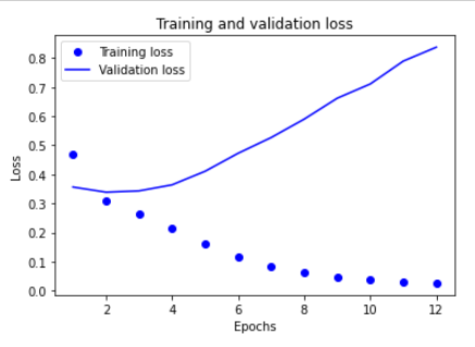
plt.clf()   # 그림을 초기화합니다

plt.plot(epochs, acc, 'bo', label='Training acc')
plt.plot(epochs, val_acc, 'b', label='Validation acc')
plt.title('Training and validation accuracy')
plt.xlabel('Epochs')
plt.ylabel('Accuracy')
plt.legend()

plt.show()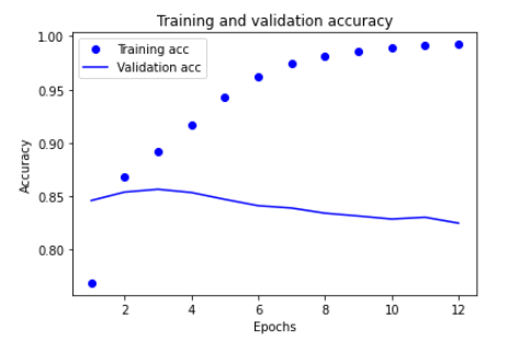
1-D CNN도 LSTM과 비슷한 그래프 모양을 하고 있습니다.
GlobalMaxPooling1D 적용해보기
model = keras.Sequential()
model.add(keras.layers.Embedding(vocab_size, word_vector_dim, input_shape=(None,)))
model.add(keras.layers.GlobalMaxPooling1D())
model.add(keras.layers.Dense(8, activation='relu'))
model.add(keras.layers.Dense(1, activation='sigmoid')) # 최종 출력은 긍정/부정을 나타내는 1dim 입니다.
model.summary()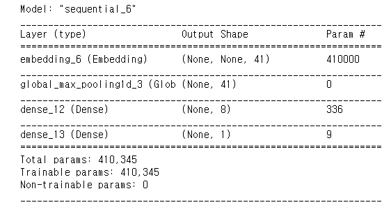
model.compile(optimizer='adam',
              loss='binary_crossentropy',
              metrics=['accuracy'])
history = model.fit(X_train,
y_train,
epochs=20,
batch_size=512,callbacks=[es],
validation_data=(X_val, y_val),
verbose=1)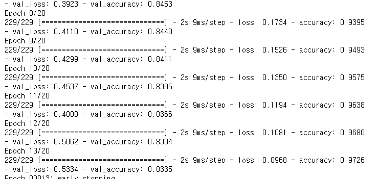
results = model.evaluate(X_test,  y_test, verbose=2)

print(results)
1537/1537 - 2s - loss: 0.5311 - accuracy: 0.8329
[0.5310723185539246, 0.8329434394836426]
GlobalMaxPooling1D그래프로 그려보기
history_dict = history.history
print(history_dict.keys())
dict_keys(['loss', 'accuracy', 'val_loss', 'val_accuracy'])
import matplotlib.pyplot as plt

acc = history_dict['accuracy']
val_acc = history_dict['val_accuracy']
loss = history_dict['loss']
val_loss = history_dict['val_loss']

epochs = range(1, len(acc) + 1)

# "bo"는 "파란색 점"입니다
plt.plot(epochs, loss, 'bo', label='Training loss')
# b는 "파란 실선"입니다
plt.plot(epochs, val_loss, 'b', label='Validation loss')
plt.title('Training and validation loss')
plt.xlabel('Epochs')
plt.ylabel('Loss')
plt.legend()

plt.show()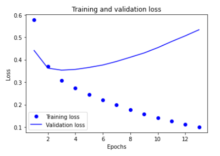
plt.clf()   # 그림을 초기화합니다

plt.plot(epochs, acc, 'bo', label='Training acc')
plt.plot(epochs, val_acc, 'b', label='Validation acc')
plt.title('Training and validation accuracy')
plt.xlabel('Epochs')
plt.ylabel('Accuracy')
plt.legend()

plt.show()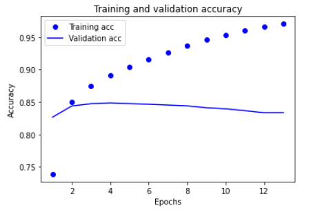
GlobalMaxPooling1D 그래프도 비슷하네요,, 그 데이터가 이런 모양이 나타나나 봅니다. cross validation을 해보고 싶어지는 그래프 모양이네요
Word2Vec 이용하기
- 비용을 절감하면서 정확도를 크게 향상시킬 수 있는 자연어처리 기법으로 단어의 특성을 저차원 벡터값으로 표현할 수 있는 word embedding 기법입니다.
[https://github.com/Kyubyong/wordvectors] 에서 공유하는 한국어 벡터값을 호출하여 사용해보도록 하겠습니다.
- 벡터값을 통해 단어들의 유사도를 더 잘 찾아줄 것이라고 기대해볼 수 있습니다.
embedding_layer = model.layers[0]
weights = embedding_layer.get_weights()[0]
print(weights.shape) # shape: (vocab_size, embedding_dim)(10000, 41)
from gensim.models import Word2Vec
import os
# 한국어 Word2Vec 사용
word2vec_path = os.getenv('HOME')+'/aiffel/sentiment_classification/data/ko.bin'
word2vec = Word2Vec.load(word2vec_path)vector = word2vec['영화']
vector영화랑 비슷한 단어가 어떤 것이 있는지 확인해 보겠습니다.
word2vec.similar_by_word("영화")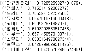
vocab_size = 10000 # 어휘 사전의 크기입니다(10,000개의 단어)
word_vector_dim = 200 # 워드 벡터의 차원수 (변경가능한 하이퍼파라미터)
embedding_matrix = np.random.rand(vocab_size, word_vector_dim)
# embedding_matrix에 Word2Vec 워드 벡터를 단어 하나씩마다 차례차례 카피한다.
for i in range(4,vocab_size):
if index_to_word[i] in word2vec:
embedding_matrix[i] = word2vec[index_to_word[i]]embedding_matrix.shapefrom tensorflow.keras.initializers import Constant
vocab_size = 10000 # 어휘 사전의 크기입니다(10,000개의 단어)
word_vector_dim = 200 # 워드 벡터의 차원 수 (변경가능한 하이퍼파라미터)
# 모델 구성
model = keras.Sequential()
model.add(keras.layers.Embedding(vocab_size,
word_vector_dim,
embeddings_initializer=Constant(embedding_matrix), # 카피한 임베딩을 여기서 활용
input_length=maxlen,
trainable=True)) # trainable을 True로 주면 Fine-tuning
model.add(keras.layers.LSTM(512)) # 가장 널리 쓰이는 RNN인 LSTM 레이어를 사용하였습니다. 이때 LSTM state 벡터의 차원수는 8로 하였습니다. (변경 가능)
model.add(keras.layers.Dense(16, activation='relu'))
model.add(keras.layers.Dense(1, activation='sigmoid')) # 최종 출력은 긍정/부정을 나타내는 1dim 입니다.
model.summary()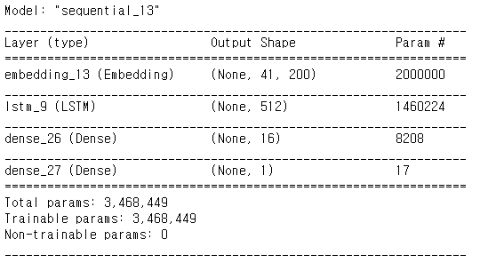
# 학습의 진행
model.compile(optimizer='adam',
              loss='binary_crossentropy',
              metrics=['accuracy'])
history = model.fit(X_train,
y_train,
epochs=20,
batch_size=256,callbacks=[es],
validation_data=(X_val, y_val),
verbose=1)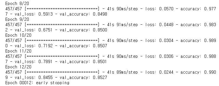
# 테스트셋을 통한 모델 평가
results = model.evaluate(X_test,  y_test, verbose=2)

print(results)
1537/1537 - 13s - loss: 0.8464 - accuracy: 0.8510
[0.8464359641075134, 0.851028323173523]
앞에서 진행한 LSTM과 큰차이는 없었지만 어쨋든 85%는 넘었네요,,, ㅎㅎ
history_dict = history.history
print(history_dict.keys())
dict_keys(['loss', 'accuracy', 'val_loss', 'val_accuracy'])
import matplotlib.pyplot as plt

acc = history_dict['accuracy']
val_acc = history_dict['val_accuracy']
loss = history_dict['loss']
val_loss = history_dict['val_loss']

epochs = range(1, len(acc) + 1)

# "bo"는 "파란색 점"입니다
plt.plot(epochs, loss, 'bo', label='Training loss')
# b는 "파란 실선"입니다
plt.plot(epochs, val_loss, 'b', label='Validation loss')
plt.title('Training and validation loss')
plt.xlabel('Epochs')
plt.ylabel('Loss')
plt.legend()

plt.show()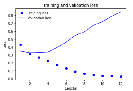
plt.clf()   # 그림을 초기화합니다

plt.plot(epochs, acc, 'bo', label='Training acc')
plt.plot(epochs, val_acc, 'b', label='Validation acc')
plt.title('Training and validation accuracy')
plt.xlabel('Epochs')
plt.ylabel('Accuracy')
plt.legend()

plt.show()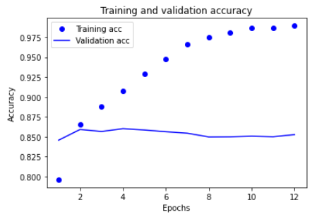
그래프를 보면서 느끼는 거지만 Validation loss는 분석이 진행할 수록 안좋아지고 정확도도 처음부터 고만고만한 정도에서 머물고 있습니다. loss가 증가하는 원인을 발견해서 최대한 막고 정확도가 올라가지 않고 유지되는 원인도 찾아서 올리면 더 좋은 강력한 모델이 만들어질 것 같습니다

잘 봤습니다! 다양한 모델을 적용해 보셨네요.
코드 블럭 앞에 python이나 py를 붙이면 하이라이팅이 됩니다. 화이팅!