14일차
- 오늘은 따로 개념적인 부분에 대한 설명은 생략
- Why??
-> 13일차에 관련 개념에 대한 설명이 되어있기 때문에
-> 오늘은 코드적으로 CNN을 구현하는 부분에 대해 기록
코드
일반적 그림
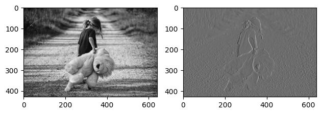
- 원본 이미지에 대해 convolution 작업을 거쳐, Feature Map을 추출한 뒤 그 결과를 확인!
# 원본 이미지에 대해 convolution 작업을 거쳐,
# Feature Map을 추출한 뒤 그 결과를 확인!

# 필요 module import
import numpy as np
import tensorflow as tf
import matplotlib.pyplot as plt
import matplotlib.image as img

# 그림을 두개 그려야 합니다
# 원본 1개, 원본에서 특성을 추출한 Feature Map 1개
fig = plt.figure()

origin = fig.add_subplot(1,2,1)
feature = fig.add_subplot(1,2,2)

img = img.imread('/content/drive/MyDrive/AI스쿨 파일/ML/girl-teddy.jpg')
origin.imshow(img)

# 원본 사진의 shape => (429, 640, 3)
img.shape

# 입력 데이터는 4차원으로 받아야 해요
# 일단, 우리의 원본 데이터를 4차원으로 변경 필요!
# (이미지 개수, height, width, color)
# (1, 429, 640, 3)
input_img = img.reshape((1,) + img.shape)  # 3차원을 4차원으로 변경하려면 이렇게 쓰면 된다!
input_img.shape  # (1, 429, 640, 3)

# 계산을 위해 픽셀값을 정수 -> 실수로
# astype() 사용해서 변경하면 된다
input_img = input_img.astype(np.float32)

# 입력이미지의 형태(shape) => (1, 429, 640, 3)
# 입력이미지의 channel을 변경해서 입력이미지의 형태를
# (1, 429, 640, 1) 이 형태로 변환할 꺼예요!
channel_1_input_img = input_img[:,:,:,0:1]  # 0:1 대신 0 사용하면 (1, 429, 640)가 되서 안됨!
channel_1_input_img.shape  # (1, 429, 640, 1)

# filter를 준비해야 해요!
# (3,3,1,1) => (filter의 height, width, filter의 channel, filter의 개수)
# 차원은 끝에서 부터 하나씩 만들어 가면 됨
filter = np.array([[[[-1]],[[0]],[[1]]],
                  [[[-1]],[[0]],[[1]]],
                  [[[-1]],[[0]],[[1]]]])

# strides => 1로 설정
# padding은 사용하지 않습니다(VALID)
conv2d = tf.nn.conv2d(channel_1_input_img,
                      filter,
                      strides=[1,1,1,1],  # 원래는 1이지만 4차원 형식 맞춰주기 위해서 이렇게 씀
                      padding='VALID')
conv2d_result = conv2d.numpy()

# featur map의 shape을 알아보아요
conv2d_result.shape

t_img = conv2d_result[0,:,:,:]  # 3차원으로 변경됨
feature.imshow(t_img, cmap='gray')

plt.tight_layout()
plt.show()- filter 부터 conv, pooling 연산까지 직접 수행
- input_img = img.reshape((1,) + img.shape)
- 이 코드를 통해 3차원을 4차원 형태로 변형할 수 있다
- 이 코드를 통해 3차원을 4차원 형태로 변형할 수 있다
- 왼쪽 원본에 대한 특징을 잡은 그림이 생성된 것을 알 수 있다
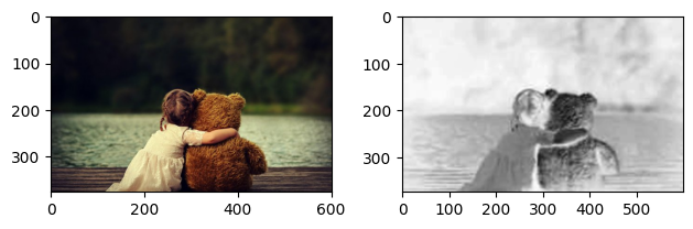
- 이번에는 원본 이미지가 컬러인 경우에 대해서 연산 수행
import numpy as np
import tensorflow as tf
import matplotlib.pyplot as plt
import matplotlib.image as img

# 그림을 두개 그려야 해요!
# 왼쪽 그림은 원본 이미지를 출력할 꺼구요!
# 오른쪽 그림은 원본에서 특징을 추출한 feature map을 출력할 꺼예요!
fig = plt.figure()

img_ori = fig.add_subplot(1,2,1)
img_feature = fig.add_subplot(1,2,2)

origin_img = img.imread('/content/drive/MyDrive/[AI_SCHOOL_9기]/images/girl-teddy-color.jpg')
img_ori.imshow(origin_img)

print(origin_img.shape)
# 원본 이미지의 shape => (376, 602, 3)

# 입력데이터는 4차원으로 표현되어야 해요!
# 우리가 이용하려는 API(Convolution연산을 수행하는 API)도
# 입력을 4차원으로 받아요!
# (이미지개수, height, width, color)
# (1, 376, 602, 3)
input_image = origin_img.reshape((1,) + origin_img.shape)
print(input_image.shape)  # (1, 376, 602, 3)
# 픽셀값을 정수에서 실수로 변환해요!
input_image = input_image.astype(np.float32)

# filter를 준비해야 해요!
# (3,3,3,1) => (filter의 hieght, filter의 width,
              # filter의 channel, filter의 개수)
filter = np.array([[[[-1], [0], [1]], [[-1], [0], [1]], [[-1], [0], [1]]],
                   [[[-1], [0], [1]], [[-1], [0], [1]], [[-1], [0], [1]]],
                   [[[-1], [0], [1]], [[-1], [0], [1]], [[-1], [0], [1]]]])
print(filter.shape)  # (3, 3, 3, 1)

# strides => 1로 설정
# padding은 사용하지 않습니다.(VALID)

conv2d = tf.nn.conv2d(input_image,
                      filter,
                      strides=[1,1,1,1],
                      padding='VALID')

conv2d_result = conv2d.numpy()

# # feature map의 shape을 알아보아요!
print(conv2d_result.shape)  #

t_img = conv2d_result[0,:,:,:]

img_feature.imshow(t_img, cmap='gray')

plt.tight_layout()
plt.show()- 컬러 이미지의 경우, 흑백과 달리 입력 이미지의 채널 수를 변경하는 과정을 생략
- 이번에는 흑백 이미지에 대해서 convolution 1번, pooling 1번을 실행한 뒤 결과 비교
# 필요 module import
import numpy as np
import tensorflow as tf
import matplotlib.pyplot as plt
import matplotlib.image as img

# 도화지 생성
fig = plt.figure()
origin = fig.add_subplot(1,3,1)
feature = fig.add_subplot(1,3,2)
pooling = fig.add_subplot(1,3,3)

# 이미지 불러오기
img = img.imread('/content/drive/MyDrive/AI스쿨 파일/ML/girl-teddy.jpg')
img.shape
origin.imshow(img)

# 원본 이미지는 3차원이에요!
# but, 입력데이터는 4차원이므로 원본을 변환해야해요
input_img = img.reshape((1,) + img.shape)
input_img.shape

# 계산을 위해 정수를 실수로 변경해요!
input_img = input_img.astype(np.float32)

# (1, 429, 640, 1)으로 변경
# why? 흑백 이미지는 channel이 1이므로 1개만 있으면 되기 때문
channel_1_input_img = input_img[:,:,:,0:1]
channel_1_input_img.shape

# filter 생성
# (3,3,1,1)
# 필터의 height, width, 필터의 channel, 개수
filter = np.array([[[[-1]],[[0]],[[1]]],
                   [[[-1]],[[0]],[[1]]],
                   [[[-1]],[[0]],[[1]]]])

# convolution 작업
conv2d = tf.nn.conv2d(channel_1_input_img,
                      filter,
                      strides=[1,1,1,1],
                      padding='VALID')
conv2d_result = conv2d.numpy()
t_img = conv2d_result[0,:,:,:]
feature.imshow(t_img,
               cmap='gray')

# pooling 작업
# 데이터의 양도 줄이면서, 특징을 좀 더 명확하게 하기 위한 방안
# kernel의 크기만 지정해주면 된다!
# 자동적으로 strides는 kernel 크기에 따라 설정되요!
# 사용하는 kernel 크기는 3 x 3으로 할꺼예요! -> 일반적으로 많이 사용?
pool = tf.nn.max_pool(conv2d_result,
                      ksize=[1,3,3,1],
                      strides=[1,3,3,1],
                      padding='VALID')
pool_result = pool.numpy()
p_img = pool_result[0,:,:,:]
pooling.imshow(p_img,cmap='gray')

plt.tight_layout()
plt.show()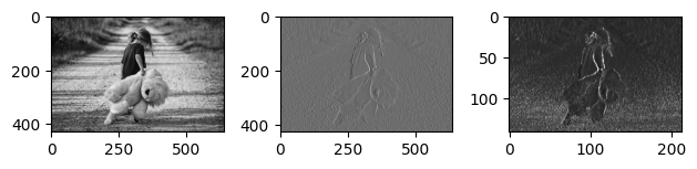
4. 3번의 pooling을 수행한 그림에 대해서 convolution을 연속해서 2번 진행하고 pooling을 1번 수행해서 결과 비교
# 필요 module import
import numpy as np
import tensorflow as tf
import matplotlib.pyplot as plt
import matplotlib.image as img

# 도화지 생성
fig = plt.figure()
ax1 = fig.add_subplot(2,3,1)
ax2 = fig.add_subplot(2,3,2)
ax3 = fig.add_subplot(2,3,3)
ax4 = fig.add_subplot(2,3,4)
ax5 = fig.add_subplot(2,3,5)
ax6 = fig.add_subplot(2,3,6)

# 이미지 불러오기
img = img.imread('/content/drive/MyDrive/AI스쿨 파일/ML/girl-teddy.jpg')
img.shape
ax1.imshow(img)

# 원본 이미지는 3차원이에요!
# but, 입력데이터는 4차원이므로 원본을 변환해야해요
input_img = img.reshape((1,) + img.shape)
input_img.shape

# 계산을 위해 정수를 실수로 변경해요!
input_img = input_img.astype(np.float32)

# (1, 429, 640, 1)으로 변경
# why? 흑백 이미지는 channel이 1이므로 1개만 있으면 되기 때문
channel_1_input_img = input_img[:,:,:,0:1]
channel_1_input_img.shape

# filter 생성
# (3,3,1,1)
# 필터의 height, width, 필터의 channel, 개수
filter = np.array([[[[-1]],[[0]],[[1]]],
                   [[[-1]],[[0]],[[1]]],
                   [[[-1]],[[0]],[[1]]]])

# convolution 작업
conv2d = tf.nn.conv2d(channel_1_input_img,
                      filter,
                      strides=[1,1,1,1],
                      padding='VALID')
conv2d_result = conv2d.numpy()
t_img = conv2d_result[0,:,:,:]
ax2.imshow(t_img,
               cmap='gray')

# pooling 작업
# 데이터의 양도 줄이면서, 특징을 좀 더 명확하게 하기 위한 방안
# kernel의 크기만 지정해주면 된다!
# 자동적으로 strides는 kernel 크기에 따라 설정되요!
# 사용하는 kernel 크기는 3 x 3으로 할꺼예요! -> 일반적으로 많이 사용?
pool = tf.nn.max_pool(conv2d_result,
                      ksize=[1,3,3,1],  # [1,3,3,1] -> 3X3을 4차원 표현 위한것으로 앞뒤 붙어있는 1은 아무 의미 X
                      strides=[1,3,3,1],
                      padding='VALID')
pool_result = pool.numpy()
p_img = pool_result[0,:,:,:]
ax3.imshow(p_img,cmap='gray')

# 여기서부터 추가되는 부분이에요!
# 우선 convolution을 2번 할거에요!
conv2d_1 = tf.nn.conv2d(pool_result,
                             filter,
                             strides=[1,1,1,1],
                             padding='VALID')
conv2d_result_1 = conv2d_1.numpy()
t1_img = conv2d_result_1[0,:,:,:]
ax4.imshow(t1_img, cmap='gray')

conv2d_2 = tf.nn.conv2d(conv2d_result_1,
                             filter,
                             strides=[1,1,1,1],
                             padding='VALID')
conv2d_result_2 = conv2d_2.numpy()
t2_img = conv2d_result_2[0,:,:,:]
ax5.imshow(t2_img, cmap='gray')

# 이제 마지막으로 pooling을 해줍시다
pool2 = tf.nn.max_pool(conv2d_result_2,
                       ksize=[1,3,3,1],
                       strides=[1,3,3,1],
                       padding='VALID')
pool2_result = pool2.numpy()
p2_img = pool2_result[0,:,:,:]
ax6.imshow(p2_img,cmap='gray')

plt.tight_layout()
plt.show()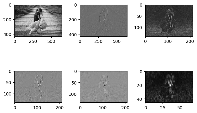
MNIST 데이터
- 이번에는 MNIST(손글씨) 데이터를 가지고 CNN 구현(tensorflow)
- 필요 라이브러리 호출
# 필요 module import
import numpy as np
import pandas as pd

from tensorflow.keras.models import Sequential
from tensorflow.keras.layers import Flatten, Dense
from tensorflow.keras.layers import Conv2D, MaxPool2D
from tensorflow.keras.optimizers import Adam

from sklearn.preprocessing import MinMaxScaler
from sklearn.model_selection import train_test_split
from sklearn.metrics import classification_report- 데이터 전처리
# Raw Data Loading
df = pd.read_csv('/content/drive/MyDrive/AI스쿨 파일/ML/MNIST/train.csv')
df

# 결측치, 이상치 없어요!
# feature engineering도 그닥 할 게 없어요!

# 데이터셋 준비
x_data = df.drop('label',axis=1,inplace=False).values
t_data = df['label'].values

# 정규화 진행
scaler = MinMaxScaler()
scaler.fit(x_data)
x_data_norm = scaler.transform(x_data)

# 데이터셋 분리
x_data_train_norm, x_data_test_norm, t_data_train, t_data_test = \
train_test_split(x_data_norm,
                 t_data,
                 stratify=t_data,
                 test_size=0.3,
random_state=0)- 모델 생성
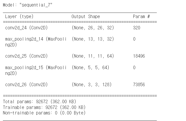
- 모델의 구조를 생각하면서 구현해보면 좀 더 쉽게 구현 가능
- 특징 추출 부분과 DNN 부분으로 구성되어 있으니 하나씩 구현
model = Sequential()

model.add(Conv2D(filters=32,  # filter의 개수
                 kernel_size=(3,3),  # filter의 크기(일반적으로 3x3 많이 사용)
                 strides=(1,1),  # strides = 1 의미
                 activation='relu',
                 input_shape=(28,28,1)))  # 하나의 이미지이기 때문에 3차원으로 변경해서
                                          # 3이 아닌 1 넣은 이유! -> shape 맞추기 위해 28*28*1 = 784

model.add(MaxPool2D(pool_size=(2,2)))

# 이미 첫번째 conv에서 input_shape 넣어줬으므로 이제 안넣어도 된다
model.add(Conv2D(filters=64,
                 kernel_size=(3,3),
                 strides=(1,1),
                 activation='relu'))

model.add(MaxPool2D(pool_size=(2,2)))

model.add(Conv2D(filters=128,
                 kernel_size=(3,3),
                 strides=(1,1),
                 activation='relu'))
model.summary()
# summary를 통해 우리가 만든 모델을 살펴볼 수 있어요!
# conv 계속할 수록 filter는 늘어남
# 작아진 이미지에서 더 많은 특징들을 잡아내겠다는 의미

# 이제 DNN 부분을 만들어봅시다!
# DNN 부분은 앞서 작성하던 방식과 비슷해요

# input layer
model.add(Flatten())  # 1차원으로 평평하게 피세요 의미!

# hidden layer
model.add(Dense(units=265,
                activation='relu'))

# output layer
model.add(Dense(units=10,
                activation='softmax'))

# model 설정
model.compile(optimizer=Adam(learning_rate=1e-3),
              loss='sparse_categorical_crossentropy',
metrics=['acc'])- 위 코드에서 onv를 더 추가 하지 않은 이유
- model.summary()를 통해 보면
-> 마지막 layer가 (None, 1, 1, 256)이 되는데 1,1은 의미가 없다!
- 모델 학습
# 모델 학습
history = model.fit(x_data_train_norm.reshape(-1,28,28,1),
                    t_data_train,
                    epochs=100,
                    batch_size=100,
                    validation_split=0.3,
                    verbose=1)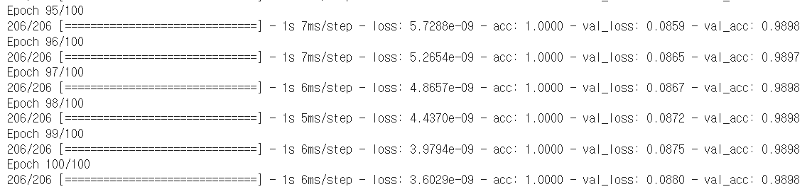
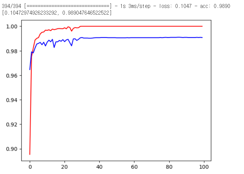
5. 평가 및 시각화
# 평가

print(model.evaluate(x_data_test_norm.reshape(-1,28,28,1),
                     t_data_test))
# [0.10472974926233292, 0.989047646522522]

# 시각화
import matplotlib.pyplot as plt

plt.plot(history.history['acc'], color='r')
plt.plot(history.history['val_acc'], color='b')

plt.show()