📖 학습주제

머신러닝, Scikit-learn, 실전 머신러닝 문제 실습 (1)

---

머신러닝 E2E(End-to-End)

주요 단계는 다음과 같다.

1. 큰 그림을 본다. (look at the big picture)
2. 데이터를 구한다. (get the data)
3. 데이터로부터 통찰을 얻기 위해 탐색하고 시각화한다. (discover and visualize the data to gain insights)
4. 머신러닝 알고리즘을 위해 데이터를 준비한다. (prepare the data for Machine Learning algorithms)
5. 모델을 선택하고 훈련시킨다. (select a model and train it)
6. 모델을 상세하게 조정한다. (fine-tune your model)
7. 솔루션을 제시한다. (present your solution)
8. 시스템을 론칭하고 모니터링하고 유지 보수한다. (launch, monitor, and maintain your system)

아래의 내용은 1990년 캘리포니아 인구조사 데이터를 기반으로 한 데이터 셋을 이용해 강의 실습에서 진행한 내용

큰 그림 보기 (Look at the Big Picture)

문제 정의

• 지도학습(supervised learning), 비지도학습(unsupervised learning), 강화학습(reinforcement learning) 중에 어떤 경우에 해당하는가?
• 분류문제(classification)인가 아니면 회귀문제(regresssion)인가?
• 배치학습(batch learning), 온라인학습(online learning) 중 어떤 것을 사용해야 하는가?

성능측정지표(performance measure) 선택

데이터 가져오기 (Get the Data)

작업환경 설정

$ export ML_PATH="$HOME/ml" # You can change the path if you prefer
$ mkdir -p $ML_PATH

$ python3 -m pip --version
pip 19.3.1 from [...]/lib/python3.7/site-packages/pip (python 3.7)

$ python3 -m pip install --user -U pip
Collecting pip
[...]
Successfully installed pip-19.3.1

독립적인 환경(isolated environment) 만들기

$ python3 -m pip install --user -U virtualenv
Collecting virtualenv
[...]
Successfully installed virtualenv-16.7.6

$ cd $ML_PATH
$ python3 -m virtualenv my_env
Using base prefix '[...]'
New python executable in [...]/ml/my_env/bin/python3
Also creating executable in [...]/ml/my_env/

$ cd $ML_PATH
$ source my_env/bin/activate # on Linux or macOS
$ .\my_env\Scripts\activate # on Windows

필요한 패키지들 설치하기

$ python3 -m pip install -U jupyter matplotlib numpy pandas scipy scikit-learn
Collecting jupyter
Downloading https://[...]/jupyter-1.0.0-py2.py3-none-any.whl
Collecting matplotlib
[...]

커널을 Jupyter에 등록하고 이름 정하기

$ python3 -m ipykernel install --user --name=python3

Jupyter 실행

$ jupyter notebook
[...] Serving notebooks from local directory: [...]/ml
[...] The Jupyter Notebook is running at:
[...] http://localhost:8888/?token=60995e108e44ac8d8865a[...]
[...] or http://127.0.0.1:8889/?token=60995e108e44ac8d8865a[...]
[...] Use Control-C to stop this server and shut down all kernels [...]

데이터 다운로드

# Python ≥3.5 is required
import sys
assert sys.version_info >= (3, 5)

# Scikit-Learn ≥0.20 is required
import sklearn
assert sklearn.__version__ >= "0.20"

# Common imports
import numpy as np
import os

# To plot pretty figures
%matplotlib inline
import matplotlib as mpl
import matplotlib.pyplot as plt
mpl.rc('axes', labelsize=14)
mpl.rc('xtick', labelsize=12)
mpl.rc('ytick', labelsize=12)

# Where to save the figures
PROJECT_ROOT_DIR = "."
CHAPTER_ID = "end_to_end_project"
IMAGES_PATH = os.path.join(PROJECT_ROOT_DIR, "images", CHAPTER_ID)
os.makedirs(IMAGES_PATH, exist_ok=True)

def save_fig(fig_id, tight_layout=True, fig_extension="png", resolution=300):
    path = os.path.join(IMAGES_PATH, fig_id + "." + fig_extension)
    print("Saving figure", fig_id)
    if tight_layout:
        plt.tight_layout()
    plt.savefig(path, format=fig_extension, dpi=resolution)

# Ignore useless warnings (see SciPy issue #5998)
import warnings
warnings.filterwarnings(action="ignore", message="^internal gelsd")

import os
import tarfile
import urllib

DOWNLOAD_ROOT = "https://raw.githubusercontent.com/ageron/handson-ml2/master/"
HOUSING_PATH = os.path.join("datasets", "housing")
HOUSING_URL = DOWNLOAD_ROOT + "datasets/housing/housing.tgz"

def fetch_housing_data(housing_url=HOUSING_URL, housing_path=HOUSING_PATH):
    if not os.path.isdir(housing_path):
        os.makedirs(housing_path)
    tgz_path = os.path.join(housing_path, "housing.tgz")
    urllib.request.urlretrieve(housing_url, tgz_path)
    housing_tgz = tarfile.open(tgz_path)
    housing_tgz.extractall(path=housing_path)
    housing_tgz.close()

fetch_housing_data를 호출하면 현재 작업공간에 datasets/housing 디렉토리를 만들고 housing.tgz 파일을 내려받고 압축을 풀어 housing.csv 파일을 만든다.

import pandas as pd

def load_housing_data(housing_path=HOUSING_PATH):
    csv_path = os.path.join(housing_path, "housing.csv")
    return pd.read_csv(csv_path)

테스트 데이터셋 만들기

• 좋은 모델을 만들기 위해선 훈련에 사용되지 않고 모델평가만을 위해서 사용될 "테스트 데이터셋"을 따로 구분하는 것이 필요
• 테스트 데이터셋을 별도로 생성할 수도 있지만 프로젝트 초기의 경우 하나의 데이터셋을 훈련, 테스트용으로 분리하는 것이 일반적

# to make this notebook's output identical at every run
np.random.seed(42)

import numpy as np

# For illustration only. Sklearn has train_test_split()
def split_train_test(data, test_ratio):
    shuffled_indices = np.random.permutation(len(data))
    test_set_size = int(len(data) * test_ratio)
    test_indices = shuffled_indices[:test_set_size]
    train_indices = shuffled_indices[test_set_size:]
    return data.iloc[train_indices], data.iloc[test_indices]

train_set, test_set = split_train_test(housing, 0.2)

• 문제점 : 새로운 데이터 추가 후 실행시, 기존의 training data가 test data로 옮겨가거나 그 반대의 일이 발생할 수 있음
• 해결방안 : 각 샘플의 식별자(identifier)를 사용해서 분할

from zlib import crc32

def test_set_check(identifier, test_ratio):
    return crc32(np.int64(identifier)) & 0xffffffff < test_ratio * 2**32

def split_train_test_by_id(data, test_ratio, id_column):
    ids = data[id_column]
    in_test_set = ids.apply(lambda id_: test_set_check(id_, test_ratio))
    return data.loc[~in_test_set], data.loc[in_test_set]

인덱스를 id로 추가

housing_with_id = housing.reset_index()   # adds an `index` column
train_set, test_set = split_train_test_by_id(housing_with_id, 0.2, "index")

• 주의사항 : Id를 만드는 데 안전한 feature들을 사용해야 함 (각 sample에 유일하게 나타나는 것들)

housing_with_id["id"] = housing["longitude"] * 1000 + housing["latitude"]
train_set, test_set = split_train_test_by_id(housing_with_id, 0.2, "id")

• Scikit-Learn에서 기본적으로 제공되는 데이터분할 함수

from sklearn.model_selection import train_test_split

train_set, test_set = train_test_split(housing, test_size=0.2, random_state=42)

계층적 샘플링(stratified sampling)

• 전체 데이터를 계층(strata)라는 동질의 그룹으로 나누고, 테스트 데이터가 전체 데이터를 잘 대표하도록 각 계층에서 올바른 수의 샘플을 추출

데이터 이해를 위한 탐색과 시각화

# 데이터 복사본 만들기 (훈련데이터를 손상시키지 않기 위해)
housing = strat_train_set.copy()

지리적 데이터 시각화

housing.plot(kind="scatter", x="longitude", y="latitude")
save_fig("bad_visualization_plot")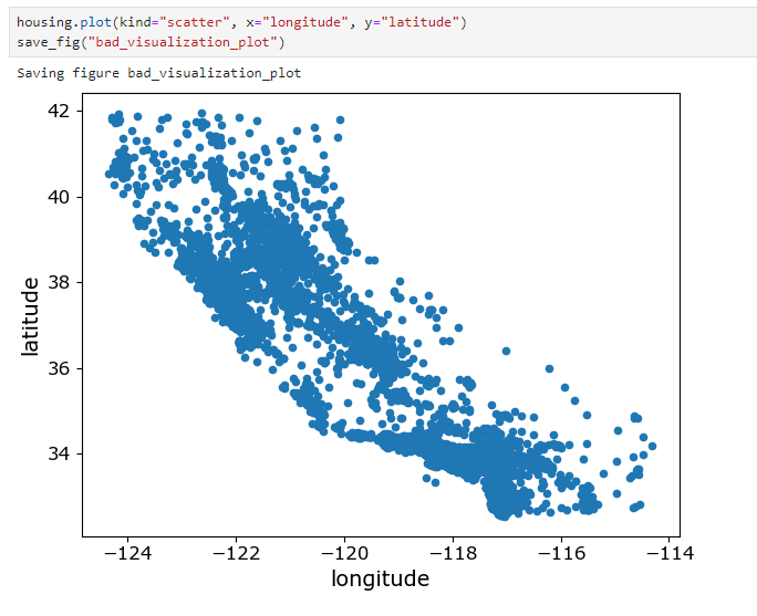

밀집된 영역 표시 : alpha옵션

housing.plot(kind="scatter", x="longitude", y="latitude", alpha=0.1)
save_fig("better_visualization_plot")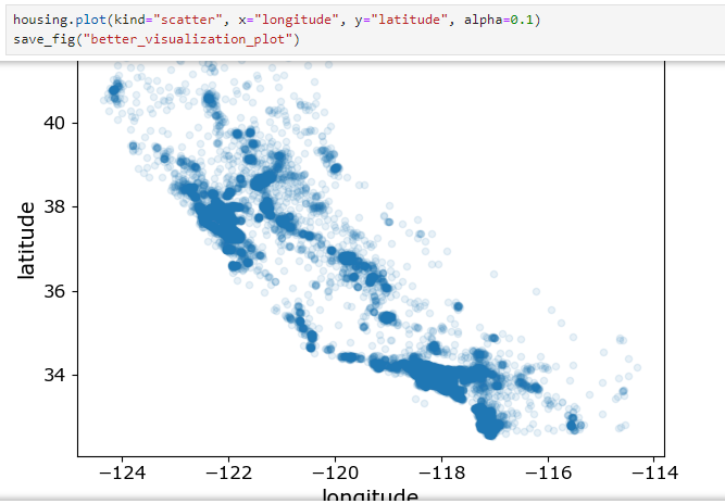

s : 원의 반지름 => 인구
c : 색상 => 가격

housing.plot(kind="scatter", x="longitude", y="latitude", alpha=0.4,
    s=housing["population"]/100, label="population", figsize=(10,7),
    c="median_house_value", cmap=plt.get_cmap("jet"), colorbar=True,
    sharex=False)
plt.legend()
save_fig("housing_prices_scatterplot")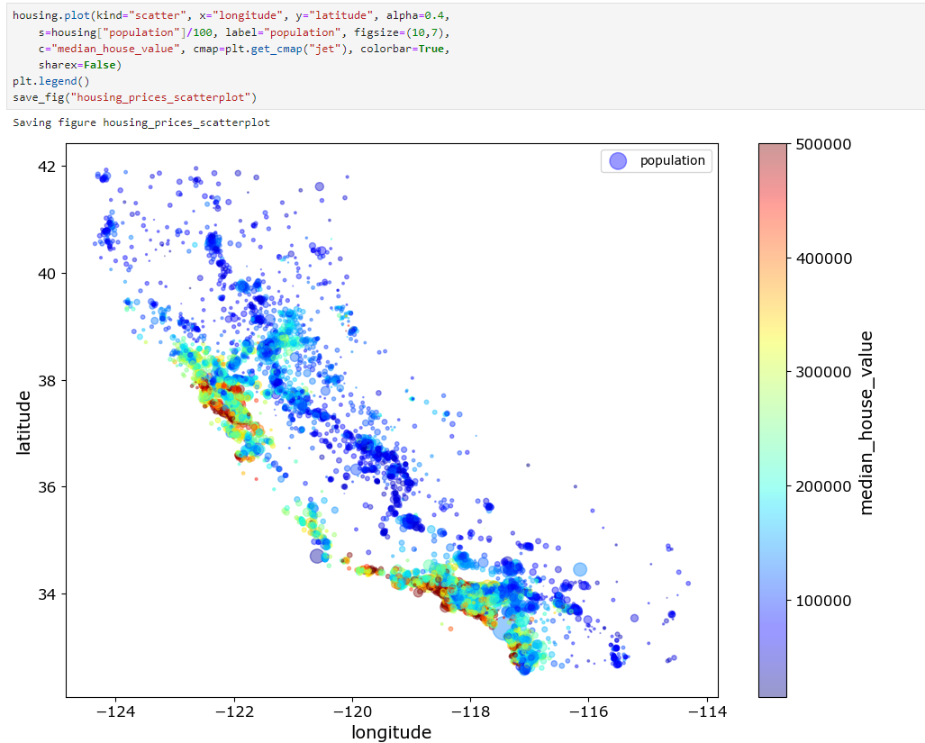

상관관계(Correlations) 관찰하기

corr_matrix = housing.corr()
corr_matrix["median_house_value"].sort_values(ascending=False)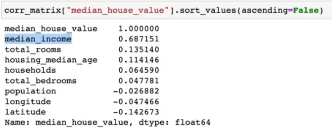

특성 조합들 실험

• 여러 특성(feature, attribute)들의 조합으로 새로운 특성을 정의해볼 수 있음
• 예를 들자면, 가구당 방 개수, 침대방(bedroom)의 비율, 가구당 인원

housing["rooms_per_household"] = housing["total_rooms"]/housing["households"]
housing["bedrooms_per_room"] = housing["total_bedrooms"]/housing["total_rooms"]
housing["population_per_household"]=housing["population"]/housing["households"]

corr_matrix = housing.corr()
corr_matrix["median_house_value"].sort_values(ascending=False)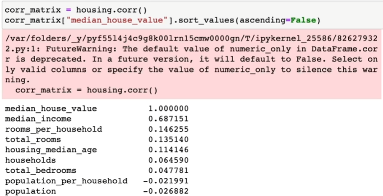

머신러닝 알고리즘을 위한 데이터 준비

데이터 준비는 데이터 변환(data transformation)과정으로 볼 수 있다.

데이터 수동변환 vs. 자동변환(함수만들기)

데이터 자동변환의 장점들

• 새로운 데이터에 대한 변환을 손쉽게 재생산(reproduce)할 수 있다.
• 향후에 재사용(reuse)할 수 있는 라이브러리를 구축하게 된다.
• 실제 시스템에서 가공되지 않은 데이터(raw data)를 알고리즘에 쉽게 입력으로 사용할 수 있도록 해준다.
• 여러 데이터 변환 방법을 쉽게 시도해 볼 수 있다.

데이터 정제(Data Cleaning)

누락된 특성(missing features) 다루는 방법들

• 해당 구역을 제거(행을 제거)
• 해당 특성을 제거(열을 제거)
• 어떤 값으로 채움(0, 평균, 중간값 등)

Estimator, Transformer, Predictor

• 추정기(estimator) : 데이터셋을 기반으로 모델 파라미터들을 추정하는 객체(e.g.) imputer). 추정자체는 fit() method에 의해서 수행되고 하나의 데이터셋을 매개변수로 전달받음(지도학습의 경우 label을 담고 있는 데이터셋을 추가적인 매개변수로 전달)

• 변환기(transformer) : (imputer같이) 데이터셋을 변환하는 추정기. 변환은 transform() method가 수행하고 변환된 데이터셋을 반환

• 예측기(predictor) : 일부 추정기는 주어진 새로운 데이터셋에 대해 예측값을 생성.(e.g.) LinearRegression) 예측기의 predict() method는 새로운 데이터셋을 받아 예측값을 반환하고고 score() method는 예측값에 대한 평가지표를 반환

Custom Transformers

• Scikit-Learn이 유용한 변환기를 많이 제공하지만 프로젝트를 위해 특별한 데이터 처리 작업을 해야 할 경우가 많은데 이 때 나만의 변환기를 만들 수 있음

반드시 구현해야 할 method들

• fit()
• transform()

특성 스케일링(Feature Scaling)

• Min-max scaling : 0과 1사이의 값이 되도록 조정
• 표준화(standardization) : 평균이 0, 분산이 1이 되도록 만들어 줌(사이킷런의 StandardScaler 사용)

변환 파이프라인(Transformation Pipelines)

• 여러 개의 변환이 순차적으로 이루어져야 할 경우 Pipeline class를 사용하면 편함
• 파이프라인의 fit() method를 호출하면 모든 변환기의 fit_transform() method를 순서대로 호출하면서 한 단계의 출력을 다음 단계의 입력으로 전달
• 마지막 단계에서는 fit() method만 호출

모델 훈련(Train a Model)

훈련 데이터셋의 RMSE가 이 경우처럼 큰 경우 => 과소적합(under-fitting)

과소적합이 일어나는 이유

• 특성들(features)이 충분한 정보를 제공하지 못함
• 모델이 충분히 강력하지 못함

모델 평가

• 테스트 데이터셋을 이용한 검증
• 훈련 데이터셋의 일부를 검증데이터(validation data)셋으로 분리해서 검증
• k-겹 교차 검증(k-fold cross-validation)

모델 세부 튜닝(Fine-Tune Your Model)

• 모델의 종류를 선택한 후에 모델을 세부 튜닝하는 것이 필요
• 모델 학습을 위한 최적의 하이퍼파라미터를 찾는 과정

그리드 탐색(Grid Search)

• 수동으로 하이퍼파라미터 조합을 시도하는 대신 GridSearchCV를 사용하는 것이 좋음

랜덤 탐색(Randomized Search)

• 하이퍼파라미터 조합의 수가 큰 경우에 유리
• 지정한 횟수만큼만 평가

특성 중요도, 에러 분석

론칭, 모니터링, 시스템 유지 보수

론칭후 시스템 모니터링

• 시간이 지나면 모델이 낙후되면서 성능이 저하
• 자동모니터링: 추천시스템의 경우, 추천된 상품의 판매량이 줄어드는지?
• 수동모니터링: 이미지 분류의 경우, 분류된 이미지들 중 일부를 전문가에게 검토시킴
  -결과가 나빠진 경우
  - 데이터 입력의 품질이 나빠졌는지? 센서고장?
  - 트렌드의 변화? 계절적 요인?

유지보수

• 정기적으로 새로운 데이터 수집(레이블)
• 새로운 데이터를 테스트 데이터로, 현재의 테스트 데이터는 학습데이터로 편입
• 다시 학습후, 새로운 테스트 데이터에 기반해 현재 모델과 새 모델을 평가, 비교

머신러닝 기초 개념들

Machine Learning (기계학습)

• 경험을 통해 자동으로 개선하는 컴퓨터 알고리즘 연구
• 학습데이터
  - 입력벡터 : $x$1, … ,$x$$N$
  - 목표값 : $t$1, … ,$t$$N$
• 머신러닝 알고리즘의 결과는 목표값을 예측하는 함수 $y$($x$)
  - $y$($x$1) ~ $t$$1$
  - $y$($x$2) ~ $t$2
  - …

($x$$i$는 $i$번째 행에 해당)

핵심개념

• 학습단계 (training/learning phase) : 함수 $y$($x$)를 학습데이터에 기반해 결정하는 단계
• 테스트 데이터셋 : 모델을 평가하기 위해서 사용하는 별도의 데이터
• 일반화 (generalization) : 모델에서 학습에 사용된 데이터가 아닌 이전에 접하지 못한 새로운 데이터에 대해 올바른 예측을 수행하는 역량
• 지도학습 (supervised learning) : 목표값(타겟, 레이블)이 주어진 경우
• 분류 (classification) : 목표값이 이산적인 경우
• 회귀 (regression) : 목표값이 연속적인 경우
• 비지도학습 (unsupervised learning) : 목표값(타겟, 레이블)이 없는 경우
• 군집 (clustering)

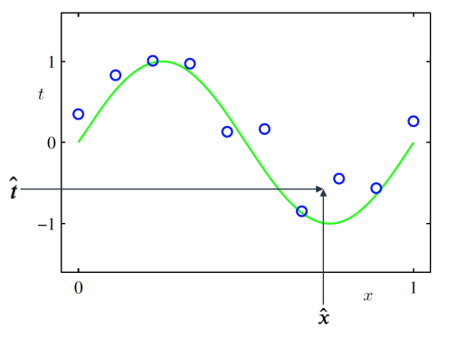
다항식 곡선 근사 (Polynomial Curve Fitting)

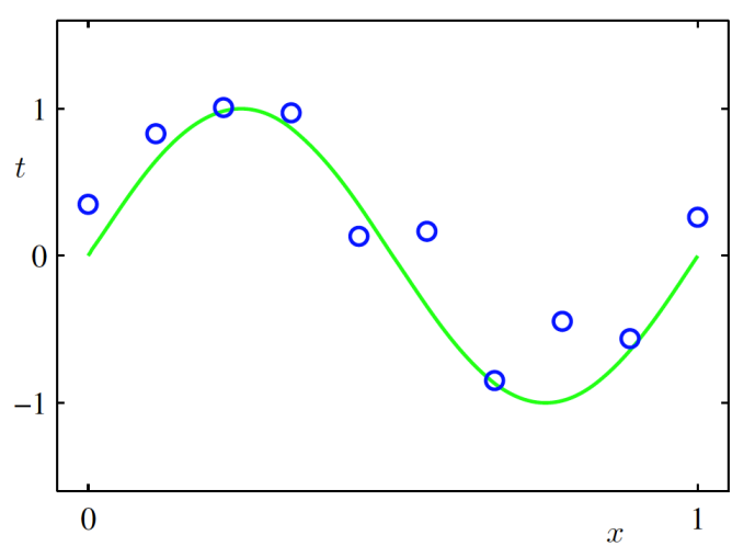
• $sin$함수가 데이터 생성
• 학습시 데이터 생성방법은 모른다고 가정

• 학습데이터 : $X$ = ($x$1, … ,$x$$N$)$T$, $t$ = ($t$1, … ,$t$$N$)$T$
• 목표 : 새로운 입력벡터$\hat{x}$가 주어졌을 때 목표값 $\hat{t}$를 예측하는 것

머신러닝에 확률이 필요한 이유

• 확률이론(probability theory) : 예측값의 불확실성을 정량화시켜 표현할 수 있는 수학적인
  프레임워크를 제공
• 결정이론(decision theory) : 확률적 표현을 바탕으로 최적의 예측을 수행할 수 있는 방법론을 제공

w 대해 선형인 다항함수

$y(x,$w$)$ = $w$0 + $w$1$x$ + $w$2$x$2 + ... $w$$M$$x$$M$ = $\displaystyle\sum_{j=0}^{M}{w_jx^j}$

오차함수 (Error Function)

주어진 w에 대한 함수값 $y$와 데이터 $t$ 사이의 차이

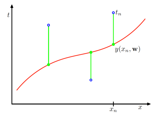
$E($w$)$ = ${1\over2}\displaystyle\sum_{n=1}^{N}{\{y(x_n,}$w${)-t_n\}^2}$를 최소화시키는 w를 구하는 것이 목표

과소적합 (Under-fitting), 과대적합 (Over-fitting)

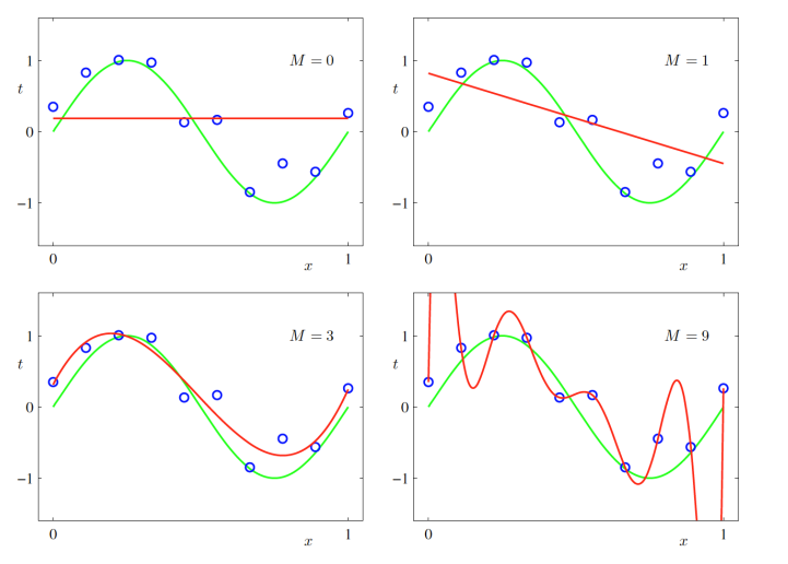
• 과소적합 : 모델이 너무 단순해서 데이터를 충분히 표현하지 못하는 경우
• 과대적합 : 모델이 너무 복잡해서 데이터의 노이즈까지 근사하려고 하는 경우

$M$ = 0, 1일 경우, 과소적합한 오차함수를 만들어 내었고, $M$ = 9일 경우, 과대적합되었다고 말할 수 있음

과소/과대적합은 모델의 일반화, 새로운 데이터에 관한 문제
-> 새로운 데이터가 들어왔을 때 오차가 클 것

이를 확인하기 위해서는 Test 데이터에 대해 오차를 구해보면 됨

$E_{RMS}$ = $\sqrt {{2E}\textbf{w}^*{/N}}$

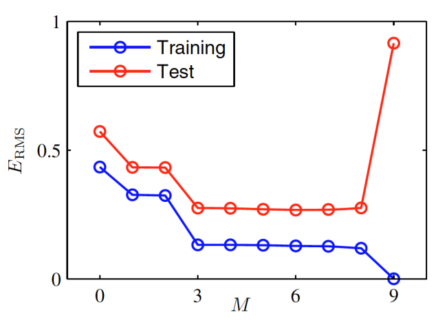
$M$이 증가함에 따라 에러가 줄어들다가 9가 되었을 때 Training 데이터에 대해서는 오차가 0이 된 반면, Test 데이터에 대해서는 오차가 갑자기 커짐을 볼 수 있음

-> 과대적합 : Training 데이터와 Test 데이터간의 오차가 크다.

아래는 $M$이 9일 때 $N$값(샘플 수)을 변경 했을 때의 결과이다.

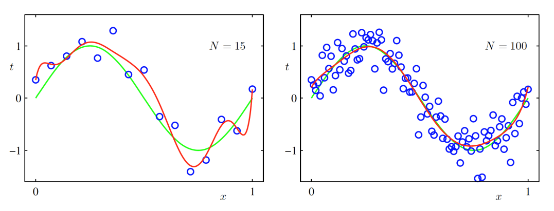
$N$값이 커지면(샘플 수가 많아지면) 점점 근사하게 됨

규제화 (Regularization)

많은 샘플 수를 확보하지 못했을 때 사용

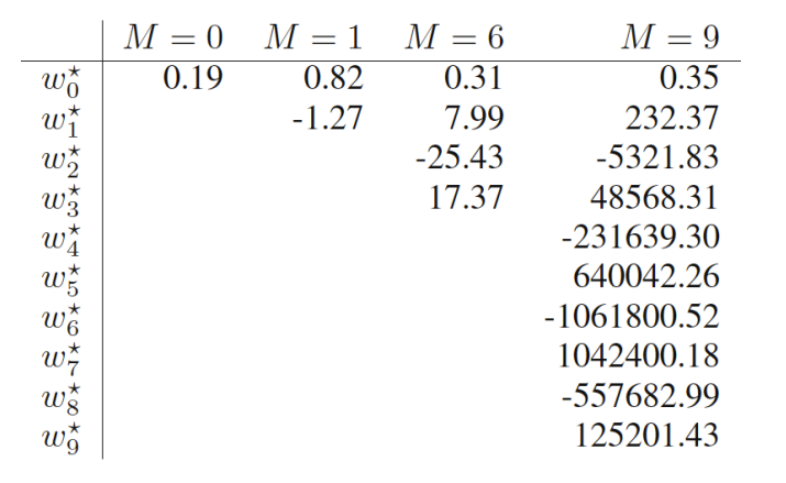
위의 그림은 $M$값마다의 최적의 파라미터 값이다.

$M$이 커져감에 따라 $w$의 값의 절대값이 커져감

이를 해결하기 위해 규제화를 이용하는데 가장 간단한 규제화의 방법 중 하나는 오차함수에 대입하는 것

새로운 오차함수를 정의한다.
$\tilde{E}($w$)$ = ${1\over2}\displaystyle\sum_{n=1}^{N}{\{y(x_n,}$w${)-t_n\}^2} + {{\lambda}\over2} {\left \| \textbf{w} \right \|}^2,$ $where$ ${\left \| \textbf{w} \right \|}^2 =$ w$T$w $= {w_0}^2 + {w_1}^2 + ... {w_M}^2$

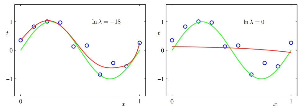
왼쪽은 어느 정도 규제화를 적용한 결과이고, 오른쪽은 기존의 문제와 동일한 경우이다.

$M$ = 9일 때

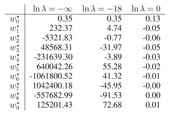
$\lambda$값을 너무 과하게 설정하면 역효과가 난다.