인공지능 2주차
AI 101 By Brandon Leshchinskiy
Google's AI-based personal assistant
Right data and right model
좋은 데이터와 모델은 많은 문제를 해결할 수 있으나 좋은 데이터를 찾고 좋은 모델로 학습시키는 것은 어렵다.
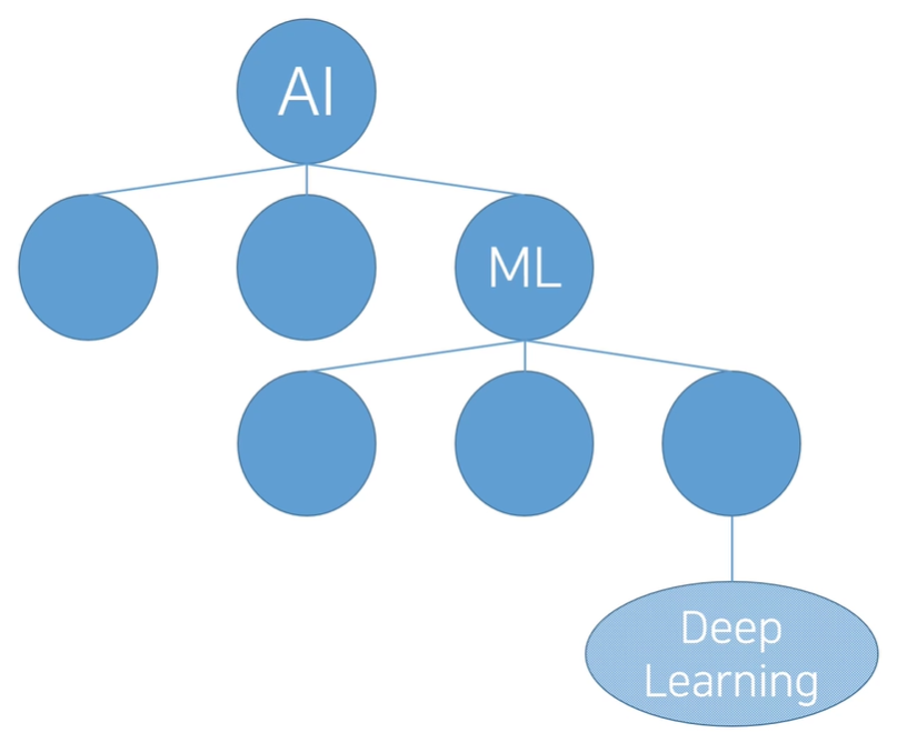
AI와 ML그리고 Deep Learning
AI는 General하거나 Narrow하다.
- Computer Vision
- Lnaguage Processing
- Planning
Expert System and tree search
- 경우의 따라서 정답을 도출하는 것
- 수많은 if-else로 구현되어 있음
Classification, Clustering, Regression
- Classification : 분류
- Clustering : 군집
- Regression : 회귀
3가지의 학습 방법
- Supervised : 지도학습
- Unsupervised : 비지도학습
- Reinforcement : 강화학습
AI Framework
- Define a Problem
- Find data
- Clean data
- Choose a model
- Train the model
- Test the model
- Deploy the model
기계 학습과 인식
Preview
- 사람은 끊임없이 주위 환경을 인식
- 타인이 말한 소리, 얼굴, 감정 등을 인식
- 생존과 자기 발전에 필수
- 주위 환경을 인식하는 인공지능
- 자율 주행차, 음성인식 챗봇, 주문 받는 로봇 등
- 이 장에서는 인식 프로그램을 만드는데 필요한 기계 학습의 기초 지식을 공부
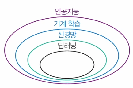
- 인공지능, 기계 학습, 신경망, 딥러닝의 관계
기계학습의 기초
- 기계 학습의 용어
- 샘플로 구성되는 데이터셋
- 특징으로 구성되는 특징 벡터(feature vector)
- 부류(class)
- 기계학습에서 데이터의 중요성
- 에너지를 만드는 연료에 해당
- 데이터가 없으면 기계학습 적용이 불가능
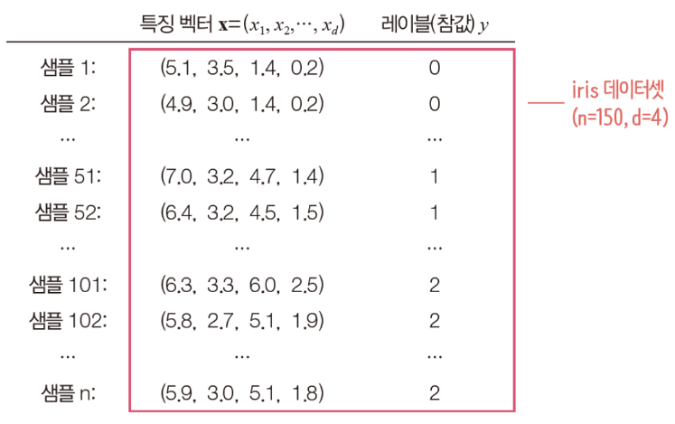
- 가장 단순한 iris 데이터로 확인해보자
데이터셋 읽기
-
사이킷런(Scikit-learn) 라이브러리 설치
pip install scikit-learn명령어로 라이브러리 설치https://sc ikit-learn.org/dev/_downloads/scikit-learn-docs.pdf에 접속하면 가장 최신 버전의 사이킷 런 사용 설명서를 무료로 다운로드할 수 있다.
-
iris 데이터셋 읽기
from sklearn import datasets

d = datasets.load.iris()	# iris 데이터셋을 읽고
print(d.DESCR)			# 내용을 출력
Iris plants dataset ------------------- **Data Set Characteristics:** # 150개의 샘플 :Number of Instances: 150 (50 in each of three classes) :Number of Attributes: 4 numeric, predictive attributes and the class :Attribute Information: # 네 개의 특징(feature) - sepal length in cm - sepal width in cm - petal length in cm - petal width in cm - class: # 세 개의 분류 - Iris-Setosa - Iris-Versicolour - Iris-Virginica :Summary Statistics: ============= === === ===== ===== ==================== Min Max Mean SD Class Correlation ============= === === ===== ===== ==================== sepal length: 4.3 7.9 5.84 0.83 0.7826 sepal width: 2.0 4.4 3.05 0.43 -0.4194 petal length: 1.0 6.9 3.76 1.76 0.9490 (high!) petal width: 0.1 2.5 1.20 0.76 0.9565 (high!) ============= === === ===== ===== ==================== :Missing Attribute Values: None :Class Distribution: 33.3% for each of 3 classes. :Creator: R.A. Fisher :Donor: Michael Marshall (MARSHALL%PLU@io.arc.nasa.gov) :Date: July, 1988# iris의 내용 살펴보기 for i in range(0, len(d.data))): # 샘플을 순서대로 출력 print(i+1, d.data[i], d.target[i]) # index, 특징 벡터, 클래스(레이블)1 [5.1 3.5 1.4 0.2] 0 2 [4.9 3.0 1.4 0.2] 0 3 [4.7 3.2 1.3 0.2] 0 4 [4.6 3.1 1.5 0.2] 0 ... 51 [7.0 3.2 4.7 1.4] 1 52 [6.4 3.2 4.5 1.5] 1 53 [6.9 3.1 4.9 1.5] 1 54 [5.5 2.3 4.0 1.3] 1 ... 101 [6.3 3.3 6.0 2.5] 2 102 [5.8 2.7 5.1 1.9] 2 103 [7.1 3.0 5.9 2.1] 2 104 [6.3 2.9 5.6 1.8] 2
기계 학습에서 데이터셋의 표현
- 샘플을 특징 벡터와 레이블로 표현
- 특징 벡터는 x로 표기(d는 특징의 개수로서 특징 벡터의 차원이라 부름)
특징 벡터 : - 레이블은 0, 1, 2, ..., c-1의 값 또는 1, 2, ..., c-1, c의 값 또는 원핫 코드
- 원핫 코드는 한 요소만 1인 이진열
예) Setosa는 (1, 0, 0), Versicolor는 (0, 1, 0), Virginica는 (0, 0, 1)
- 원핫 코드는 한 요소만 1인 이진열
- 특징 벡터는 x로 표기(d는 특징의 개수로서 특징 벡터의 차원이라 부름)
기계 학습 적용: 모델링과 예측
-
기계 학습 모델 : SVM(Support vector machine)
from sklearn import svm
s = svm.SVC(gamma=0.1, C=10)	# 하이퍼 매개변수
s.fit(d.data, d.target)		# 훈련 집합, fit은 훈련시키는 함수

new_d = [[6.4, 3.2, 6.0, 2.5], [7.1, 3.1, 4.7, 1.35]]

res = s.predict(new_d)		# 테스트 집합
print("새로운 2개 샘플의 부류는", res)
새로운 2개 샘플의 부류는 [2, 1] -
훈련 집합(Training Set)과 테스트 집합(Test Set)
- 훈련 집합: 기계 학습 모델을 학습하는데 쓰는 데이터로서 특징 벡터와 레이블 정보를 모두 제공
- 테스트 집합: 학습을 마친 모델의 성능을 측정하는데 쓰는 데이터로서 예측할 때는 특징 벡터 정보만 제공하고, 예측 결과를 가지고 정확률을 측정할 때 레이블 정보를 사용
- 하이퍼 매개변수 설정: 하이퍼 매개변수(Hyper parameter)란 모델의 동작을 제어하는데 쓰는 변수이다. 모델의 학습을 시작하기 전에 설정해야 하는데, 적절한 값을 설정해야 좋은 성능을 얻을 수 있다. 최적의 하이퍼 매개변수 값을 자동으로 설정하는 일을 하이퍼 매개변수 최적화(hyper parameter optimization)라 하는데, 이것은 기계 학습의 중요한 주제 중 하나이다.
인공지능 제품의 설계와 구현
-
인공지능 제품의 핵심
- 데이터를 읽고 모델링과 예측을 수행
- 붓꽃 영상을 획득하고 특징을 추출하는 컴퓨터 비전 모듈을 전처리로 붙이면 붓꽃 인식 프로그램 완성
-
실용적인 시스템 사례
- 과일 등급 분류
- 딸기 따는 로봇
- 위 모두의 과정을 따르는 로봇
-
인공지능 설계 사례: 과일 등급을 분류하는 기계
- 사과를 상중하의 세 부류로 분류하는 인공지능 기계의 설계
- 데이터 확보
- 상중하 비율이 비슷하게 수천 개의 사과 수집(데이터 편향:data bias을 방지하기 위해 여러 농장에서 수집)
- 카메라로 촬영하여 파일에 저장
- 데이터 편향: 데이터 편향은 다양한 형태로 발생한다. 예를 들어 필기 숫자 데이터셋을 만들 때 편의상 대학생을 대상으로 수집했다면 정자체에 가까운 샘플의 비율이 높을 수 있다. 은행 창구에서 발생하는 전표나 우편 봉투에 쓰인 우편번호에서 수집하면 데이터 편향을 크게 줄일 수 있다.
- 특징 벡터와 레이블 준비
- 어떤 특징을 사용할까? 예) 사과의 크기, 색깔, 표면의 균일도는 분별력이 높은 특징
- 컴퓨터 비전 기술로 특징 추출 프로그램 작성, 특징 추출하여 apple.data 파일에 저장
- 사과 분류 전문가를 고용하여 레이블링, apple.target 파일에 저장
- 학습하는 과정을 프로그래밍(훈련 데이터 사용)
from sklearn import svm s = svm.SVC(gamma=0.1, C=10) s.fit(apple.data, apple.target) # apple 데이터로 모델링 - 예측 과정을 프로그래밍(새로 수집한 테스트 데이터 사용)
s.predict(x) # 새로운 사과에서 추출한 특징 벡터 x를 예측
- 데이터 확보
- 사과를 상중하의 세 부류로 분류하는 인공지능 기계의 설계
규칙 기반 vs 고전적 기계 학습 vs 딥러닝
- 규칙 기반 방법
- 분류하는 규칙을 사람이 구현하는 방법
- 예) "꽃잎의 길이가 a보다 크고, 꽃잎의 너비가 b보다 작으면 Setosa"라는 규칙에서 a, b를 사람이 결정해 줌
- 기계 학습 방법
- 특징 벡터를 추출하고 레이블을 붙이는 과정은 규칙 기반과 동일(수작업 특징: hand-crafted feature)
- 규칙 만드는 일은 기계학습 모델을 이용하여 자동으로 수행
- 딥러닝 방법
- 레이블을 붙이는 과정은 기계 학습과 동일
- 특징 벡터를 학습이 자동으로 알아냄. 특징 학습(feature learning) 또는 표현 학습(representation learning)을 한다고 말함
- 장점
- 특징 추출과 분류를 동시에 최적화하므로 뛰어난 성능 보장
- 인공지능 제품 제작이 빠름
머신러닝이란 무엇인가?
- 머신러닝이란 데이터를 통해 알 수 있는 컴퓨터 과학이다.
- 일반화된 정의: Rule이라는 것을 명시하지 않고 학습시키는 것
- 공학적인 접근: 주어진 목표인
T를 위해 경험을 통해 학습하고ET를 통해 성능 평가를 하는 것P또한 주어진T를 통해 더욱 향상시키는 것 (Tom Mitchell, 1997)
Classes of Learning Problem
- Supervised Learning
- Data: (x, y)
x = data, y = label - Goal: Learn function to map
X → Y - Apple Example

- Data: (x, y)
- Unsupervised Learning
- Data: x
x = data, no label - Goal: Learn underlying structure
- Apple Example
- Data: x
- Reinforcement Learning
- Data: (state-action) pairs
- Goal: Maximize future rewards over many time steps
- Apple Example

특징 공간에서 데이터 분포
- iris 데이터
-
특징이 4개이므로 4차원 특징 공간을 형성
-
150개 샘플 각각은 4차원 특징 공간의 한 점
-
차원을 하나 제외하고 3차원 공간에 데이터 분포를 그림
# iris 데이터의 분포를 특징 공간에 그리기
import plotly.express as px

df = px.data.iris()
fig = px.scatter_3d(df, x='sepal_length', y='sepal_width', z='petal_width' color='species')
fig.show(rendere="browser")
-
- 특징 공간에서 데이터 분포 관찰
- petal width(수직 축)에 대해 Setosa는 아래쪽, Virginica는 위쪽에 분포 즉, petal width 특징은 분별력(discriminating power)이 뛰어남
- sepal width 축은 세 부류가 많이 겹쳐서 분별력이 낮음
- 전체적으로 보면, 세 부류가 3차원 공간에서 서로 다른 영역을 차지하는데 몇 개 샘플은 겹쳐 나타남
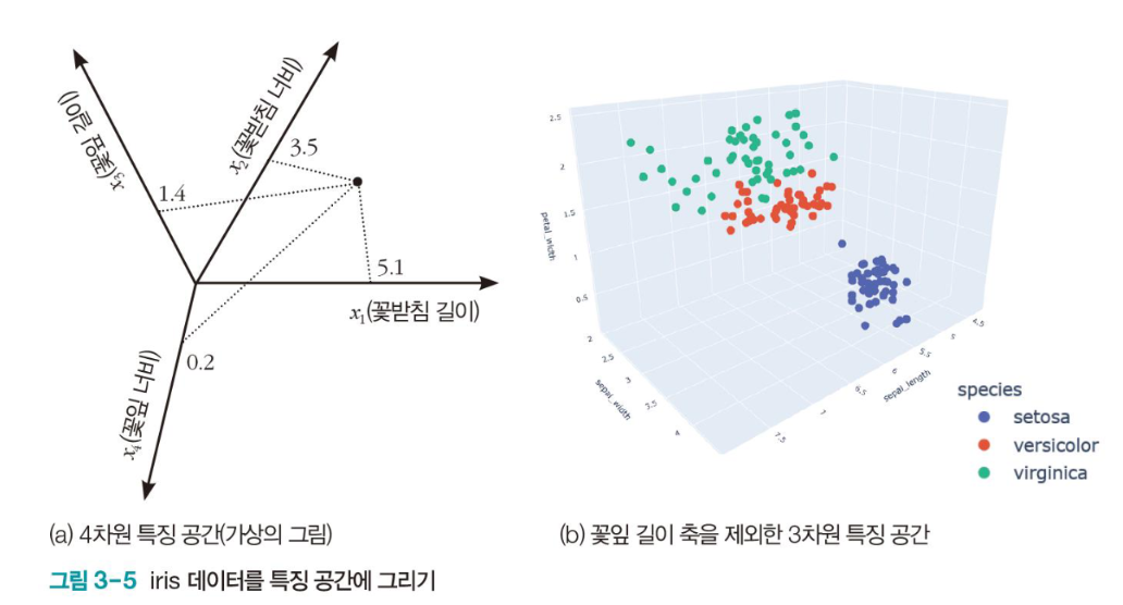
- Feature Space를 통해 Setosa를 잘 분류할 수 있다는 것을 파악가능
영상 데이터 사례: 필기 숫자
-
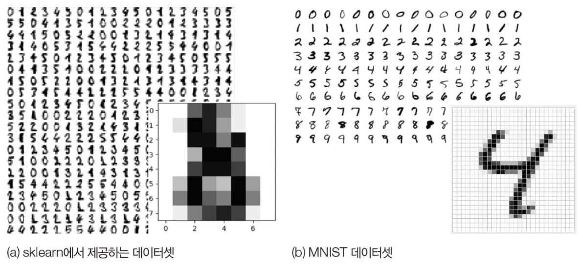
두 가지 필기 숫자 데이터셋
-
sklearn 데이터셋: 8*8맵(64개 화소), 1797개 샘플, [0, 16]명암값
-
MNIST 데이터셋: 28*28맵(784개 화소), 7먄개 샘플, [0, 255]명암값
from sklearn import datasets
import matplotlib.pyplot as plt

digit.datasets.load_digits()

plt.figure(figsize=(5,5))
plt.imshow(digit.images[0], cmap=plt.cm.gray_r, interpolation='nearest')

plt.show()
print(digit.data[0])
print("이 숫자는 ", digit.target[0], "입니다.")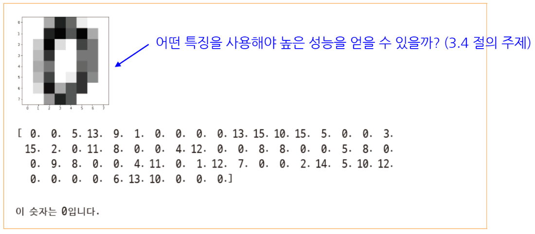
-
텍스트 데이터 사례: 20newsgroups
-
20newsgroups 데이터셋
- 웹에서 수집한 문서를 20개 부류로 구분, 텍스트로 구성되어 샘플의 길이가 다름
- 시계열 데이터(단어가 나타나는 순서가 중요. 8장의 순환 신경망에서 다룸)
news = datasets.fetch.20newsgroups(subset="train")	# 데이터셋 열기
print("-----\n', news.data[0], "\n-----")
print("이 문서의 부류는 <", news.target.names[news[news.target[0]], "> 입니다.")
***** From: lerxst@wam.umd.edu (where's my thing) Subject: WHAT car is this!? Nntp-Posting-Host: rac3.wam.umd.edu Organization: University of Maryland, College Park Lines: 15 I was wondering if anyone out there could enlighten me on this car I saw the other day. It was a 2-door sports car, looked to be from the late 60s/ early 70s. It was called a Bricklin. The doors were really small. In addition, the front bumper was separate from the rest of the body. This is --- ***** 이 문서의 부류는 < rec.autos >입니다.
특징 추출과 표현
- 기계 학습의 전형적인 과정
- 실제에서는 다양한 형태로 나타남
데이터 수집→특징 추출→모델링→예측
- 실제에서는 다양한 형태로 나타남
특징의 분별력
- 사람은 직관적으로 분별력(discriminating power)이 높은 특징을 사용
- 예) 두 텀블러를 구분하는 특징
- 글씨 방향, 몸통 색깔, 손잡이 유무, 뚜껑 유무 등
- 뚜껑 유무라는 특징은 분별력이 없음
- 손잡이 유무라는 특징은 높은 분별력
- 기계 학습은 높은 분별력을 지닌 특징을 사용해야 함
- 예) 100여년 전의 iris 데이터는 사람이 네 종류의 특징을 자를 들고 직접 추출
- 현대에서는 붓꽃 영상을 그대로 입력하면 딥러닝이 최적의 특징을 추출해 줌
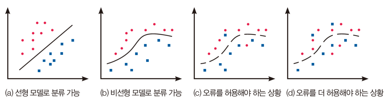
- 다양한 형태의 특징 공간
- 실제 세상은 비선형 데이터[(c)~(d)]를 생성(데이터의 원천적인 성질 또는 측정이나 레이블링 오류, 비합리적인 특징 추출 알고리즘에 기인)
- 가급적 (d)보다는 (c)와 같은 특징을 사용해야 함.
특징 값의 종류
- 수치형 특징
- 예) iris의 네 개 특징은 실수
- 거리 개념이 있음
- 실수 또는 정수 또는 이진값
- 범주형 특징
- 순서형: 학점, 수능 등급 등
- 거리 개념이 있음, 순서대로 정수를 부여하면 수치형으로 취급 가능
- 이름형
- 혈액형, 지역 등으로 거리 개념이 없음
- 보통 원핫(one-hot)코드로 표현 예) A형(1, 0, 0, 0) B형(0, 0, 1, 0)...
- 순서형: 학점, 수능 등급 등
필기 숫자 인식
- 절차에 따라 필기 숫자 데이터셋을 가지고 프로그래밍 연습
- 특징 추출을 위한 코드 작성
- sklearn이 제공하는 fit함수로 모델링(학습)
- predict 함수로 예측
필기 숫자 인식
- 화소 각각을 특징으로 간주
- sklearn의 필기 숫자는 8*8맵으로 표현되므로 64차원 특징 벡터
- 2차원 구조를 1차원 구조로 변환
- 예)
x = (0,0,5,13,9,1,0,0,0,0,13,15,10,15... 64개의 특징 벡터)
화소 값을 특징으로 사용
from sklearn import datasets
from sklearn import svm

digit=datasets.load_digits()

# svm의 분류기 모델 SC를 학습
s=svm.SVC(gamma=0.1, C=10)
s.fit(digit.data, digit.target) # digit 데이터로 모델링

# 훈련 집합의 앞에 있는 샘플 3개를 새로운 샘플로 간주하고 인색해봄
new_d = [digit.data[0], digit.data[1], digit.data[2]]
res = s,predict(new_d)
print("예측값은", res)
print("참값은", digit.target[0], digit.target[1], digit.target[2])

# 훈련 집합을 테스트 집합으로 간주하여 인식해보고 정확률을 측정
res = s.predict(digit.data)
correct=[i for i in range(len(res)) if res[i]==digit.targe[i]]
accuracy=len(correct)/len(res)
print("화소 특징을 사용했을 때 정확률=", accuracy*100, "%")
예측값은 [0 1 2]
참값은 0 1 2
화소 특징을 사용했을 때 정확률=100.0%성능 측정
- 객관적인 성능 측정의 중요성
- 모델 선택할 때 중요
- 현장 설치 여부 결정할 때 중요
- 일반화(generalizaiton) 능력
- 학습에 사용하지 않았던 새로운 데이터에 대한 성능
- 가장 확실한 방법은 실제 현장에 설치하고 성능 측정 → 비용 때문에 실제 적용 어려움
- 주어진 데이터를 분할하여 사용하는 지혜 필요
혼동 행렬과 성능 측정 기준
- 혼동 행렬(Confusion matrix)
- 부류 별로 옳은 분류와 틀린 분류의 개수를 기록한 행렬
- 는 모델이 라고 예측했는데 실제 부류는 인 샘플의 개수
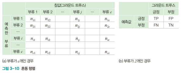
- 이진 분류에서 긍정(Positive)과 부정(negative)
- 참 긍정(TP), 거짓 부정(FN), 거짓 긍정(FP), 참 부정(TN)의 네 경우
- 널리 쓰이는 성능 측정 기준
- 정확률(accuracy)
- 부류가 불균형일 때 성능을 제대로 반영하지 못함
정확률 - 특이도(Specificity)와 민감도(Sensitivity) : 주로 의료에서 사용
특이도 민감도 - 정밀도(Precision)와 재현률(recall) : 주로 정보검색에서 사용
정밀도 재현율
- 부류가 불균형일 때 성능을 제대로 반영하지 못함
- 정확률(accuracy)
훈련/검증/테스트 집합으로 쪼개기
-
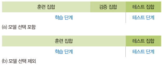
주어진 데이터를 적절한 비율로 훈련, 검증, 테스트 집합으로 나누어 씀
- 모델 선택 포함: 훈련/검증/테스트 집합으로 나눔
- 모델 선택 제외: 훈련/테스트 집합으로 나눔
from sklearn import datasets from sklearn import svm from sklearn.model_selection import train_test_split # 데이터셋을 읽고 훈련 집합과 테스트 집합으로 분할 digit = datasets.load_digits() x_train, x_test, y_train, y_test = train_split(digit.data, digit.target, train_size=0.6) # svm의 분류 모델 SVC를 학습 s = svm.SVC(gamma=0.001) s.fit(x_train, y_train) res = s.predict(x_test) # 혼동 행렬 구함 conf=np.zeros((10,10)) for i in range(len(res)): conf[res[i]][y_test[i]] += 1 print(conf) # 정확률 측정하고 출력 no_correct = 0 for i in range(10): no_correct += conf[i][i] accuracy=no_correct/len(res) print("테스트 집합에 대한 정확률은", accruracy*100, "%입니다.") -
난수를 사용하기 때문에 실행할 때마다 다른 결과가 나오는 프로그램
- 위 코드는 실행할 때마다 출력이 다르게 나온다. train_test_split 함수가 난수를 사용해 데이터를 분할하기 때문이다. 앞으로 등장하는 프로그램에서도 난수를 사용하는 경우가 있는데 마찬가지로 실행할 때마다 다른 결과를 얻게 된다. 동일한 실행 결과를 얻으려면 이전에 np.random.seed(0)을 추가하면 된다. 매개변수 0은 다른 값을 사용해도 된다. 어떤 값이든 고정시키면 매번 같은 난수 열이 생성된다.
교차 검증
-
훈련/테스트 집합 나누기의 한계
- 우연히 높은 정확률 또는 우연히 낮은 정확률 발생 가능성
-
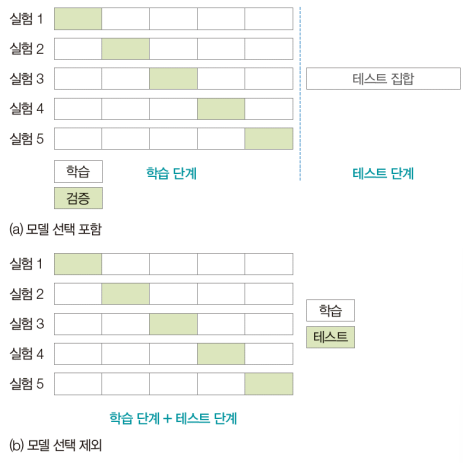
k-겹 교차 검증
- 훈련 집합을 k개의 부분집합으로 나누어 사용. 한 개를 남겨두고 k-1개로 학습한 다음 남겨둔 것으로 성능 측정, k개의 성능을 평균하여 신뢰도 높임
- 훈련 집합을 k개의 부분집합으로 나누어 사용. 한 개를 남겨두고 k-1개로 학습한 다음 남겨둔 것으로 성능 측정, k개의 성능을 평균하여 신뢰도 높임
-
digit 데이터에 교차 검증 적용
- cross_val_score 함수가 교차 검증 수행해줌(cv=5는 5-겹 교차 검증하라는 뜻)
- 실행 결과 정확률이 들쭉날쭉. 한번만 시도하는 [프로그램 3-5]의 위험성을 잘 보여줌
- k를 크게 하면 신뢰도 높아지지만 실행 시간이 더 걸림
from sklearn import datasets
from sklearn import svm
from sklearn.model_selection import cross_val_score
import numpy as np

digit=datasets.load_digits()
s=svm.SVC(gamma=0.001)
accuracies=cross_val_score(s, digit.data, digit.target, cv=5)	# 5-겹 교차 검증

print(accuracies)
print("정확률(평균)=%0.3f, 표준편차=%0.3f"%(accuracies.mean()*100, accuracies.std()))
[0.97527473 0.95027624 0.98328691 0.99159664 0.95774648] 정확률(평균)=97.164, 표준편차=0.015
인공지능은 어떻게 인식을 하나?
- 지금까지는 모델(분류기)의 원리에 대한 이해없이 프로그래밍 실습
- 지금까지 기계 학습 모델인 SVM을 블랙 박스로 보고 프로그래밍
- 동작 원리에 대한 이해 없으면 언젠가 한계가 드러남
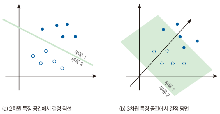
특징 공간을 분할하는 결정 경계
-
인공지능의 인식은 철저히 수학에 의존
- 샘플은 특징 벡터로 표현되며, 특징 벡터는 특징 공간의 한 점에 해당
- 인식 알고리즘은 원래 특징 공간을 성능을 높이는데 더 유리한 새로운 특징 공간으로 여러 차례 변환한 다음 최종적으로 특징 공간을 분할하여 부류를 결정
- 특징 공간 변환 예
- 원래 특징 공간 →
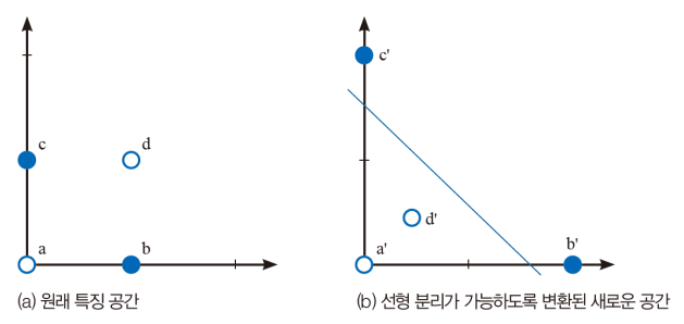
- 원래 특징 공간 →
-
특징 공간을 분할하는 결정 경계(decision boundary)
- 2~3차원은 그림을 그릴 수 있는데 4차원 이상은 수학적 상상력 필요
- 2~3차원은 그림을 그릴 수 있는데 4차원 이상은 수학적 상상력 필요
-
현대 기계 학습이 다루는 데이터
- 수백~수만 차원 특징 공간
- 고차원 공간에서 부류들이 서로 꼬여있는 매우 복잡한 분포
- 딥러닝은 층을 깊게 하여 여러 단계의 특징 공간 변환을 수행(특징 학습 또는 표현 학습이라 부름)
-
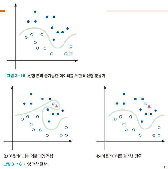
결정 경계를 정하는 문제에서 고려 사항
- 비선형 분류기(nonlinear classifier) 사용
- 과잉 적합 overfitting 회피
- 과잉 적합은 아웃라이어를 맞히려고 과다하게 복잡한 결정 경계를 만드는 형상
- 훈련 집합에 대한 성능은 높지만 테스트 집합에 대해서는 형편없는 성능(낮은 일반화)
- 원인과 대처법 또한 존재
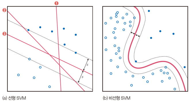
SVM의 원리
- SVM의 동기
- 100% 정확률인 두 분류기 ②와 ③은 같은가?
- 100% 정확률인 두 분류기 ②와 ③은 같은가?
- 기계 학습의 목적은 일반화 능력을 극대화하는 것
- SVM은 일반화 능력을 높이려 여백을 최대화
- 분류기 ②는 빨간색 부류에 조금만 변형이 생겨도 결정 경계를 넘을 가능성. ③은 두 부류 모두에 대해 멀리 떨어져 있어 경계를 넘을 가능성이 낮음
- SVM은 두 부류까지의 거리인 2s를 여백이라 부름. SVM 학습 알고리즘은 여백을 최대화하는 결정 경계를 찾음
- SVM을 비선형 분류기로 확장
- 원래 SVM은 선형 분류기
- 커널 트릭을 사용하여 비선형 분류기로 확장(커널 함수를 사용하여 선형 공간을 비선형 공간으로 변형)
- 커널 함수로는
polynomial function,radial basis function,sigmoid함수를 사용- 커널 함수의 종류와 커널 함수의 모양을 조절하는 매개변수는 하이퍼 매개변수
- C라는 하이퍼 매개변수
- 지금까지 모든 샘플을 옳게 분류하는 경우를 다룸. 실제로는 오류를 허용하는 수밖에 없음
- C를 크게 하면, 잘못 분류한 훈련 집합의 샘플을 적은데 여백이 작아짐(훈련 집합에 대한 정확률은 높지만 일반화 능력 떨어짐)
- C를 작게 하면, 여백은 큰데 잘못 분류한 샘플이 많아짐(훈련 집합에 대한 정확률은 낮지만 일반화 능력 높아짐)
- 커널 트릭을 사용하여 비선형 분류기로 확장(커널 함수를 사용하여 선형 공간을 비선형 공간으로 변형)
- 커널 함수로 기본값 rbf를 사용. gamma는 rbf 관련한 매개변수
- C=10 사용
s=svm.SVC(gamma=0.1, C=10)