자음 인식 모델_V2

지난 번 사용했던 모델의 경우 파라미터의 개수가 2백4십만여개에 약 98%의 정확도를 보였다.
CNN모델의 경우, 대체적으로 네트워크가 깊어질수록 더 높은 정확도를 보인다고 하는데, 이번에는 모델을 수정하여 파라미터의 수도 줄이고 정확도도 높여보려고 한다.

import tensorflow.keras
from tensorflow.keras.models import Model
from tensorflow.keras.layers import Conv2D, MaxPool2D, Dropout, Dense, Input, \
    concatenate, AveragePooling2D, Flatten
import tensorflow.keras
import cv2
from sklearn.model_selection import train_test_split
from glob import glob
import numpy as np

모델 학습에 사용할 데이터는 지난 번과 마찬가지로 14개 자음 데이터이며, 64x64이미지가 아닌 96x96이미지로 학습시킬 예정이다.

먼저, 데이터를 불러오자.

def load_data(imgHeight, imgWidth):
    path = '이미지 경로'  
    categories = ["ㄱ", "ㄴ", "ㄷ", "ㄹ","ㅁ", "ㅂ","ㅅ", "ㅇ",
        "ㅈ", "ㅊ","ㅋ", "ㅌ","ㅍ","ㅎ"]
    nb_categories = len(categories)
    X = []
    y = []
    count = 0

    for idx, correct in enumerate(categories):
        label = [0 for i in range(nb_categories)]
        label[idx] = 1
        files = glob(path + correct + '/*')
        print(path + correct + '/')

        for f in files:
            img = imread(f)
            img = cv2.cvtColor(img, cv2.COLOR_BGR2GRAY)
            img = cv2.resize(img, (imgWidth, imgHeight))
            data = np.asarray(img)
            X.append(data)
            y.append(label)
            count += 1

    X = np.array(X)
    y = np.array(y)
    X = X.reshape(count, imgHeight, imgWidth, 1)

    X_train, X_test, y_train, y_test = train_test_split(X, y, test_size=0.3, shuffle=True, stratify=y, random_state=34)
    X_train = X_train.astype('float64') / 255
    X_test = X_test.astype('float64') / 255
    return nb_categories, X_train, y_train, X_test,y_test

인식 모델은 아래와 같이 작성하였는데, 지난 번과 달라진 점으로는 Sequential API로 네트워크를 구성한 것이 아닌, Functional API를 사용했다는 점과, inception_module을 사용했다는 점이다.

구글 LeNet의 경우 inception_module을 여러 번 사용하였으며 중간 단계에서 Softmax로 예측하는 부분이 있는데, 필자는 inception_module을 한 번만 사용하여 중간 단계에서 에측하는 부분은 제외하였다. padding을 same으로 하여 필터의 크기와 stride의 크기를 임의로 조정하여 마지막 maxpool2D()연산 이후 feature-map의 크기를 의도적으로 1x1이 되게 하여, flatten()시 파라미터의 수가 증가하지 않도록 해보았다.

def inception_module(x, filters_1x1, filters_3x3, name=None):
    branch_a = Conv2D(filters_1x1, (1,1), padding='same', activation='relu', strides=2)(x)

    branch_b = Conv2D(filters_1x1, (1,1), padding='same', activation='relu')(x)
    branch_b = Conv2D(filters_3x3, (3,3), padding='same', activation='relu', strides=2)(branch_b)

    branch_c = AveragePooling2D((3,3), padding='same', strides=1)(x)
    branch_c = Conv2D(filters_3x3, (3,3), padding='same', activation='relu', strides=2)(branch_c)

    branch_d = Conv2D(filters_1x1, (1,1), padding='same', activation='relu')(x)
    branch_d = Conv2D(filters_3x3, (3,3), padding='same', activation='relu')(branch_d)
    branch_d = Conv2D(filters_3x3, (3,3), padding='same', activation='relu', strides=2)(branch_d)

    output = concatenate([branch_a, branch_b, branch_c, branch_d], axis=3, name=name)
    return output

def main():
    imgWidth = 96
    imgHeight = 96
    nb_categories, X_train, y_train, X_test,y_test = load_data(imgHeight, imgWidth)
    input_layer = Input(shape=(imgHeight, imgWidth, 1))
    
   #Layer1
    x = Conv2D(8, (3, 3), padding='same', strides=(1, 1), activation='relu', name='conv_1_3x3/1')(input_layer)
    x = MaxPool2D((3, 3), strides=(2, 2), name='max_pool_1_3x3/1', padding='same')(x)

    #Layer2
    x = Conv2D(16, (3, 3), padding='same', strides=(1, 1), activation='relu', name='conv_2_3x3/2')(x)
    x = MaxPool2D((3, 3), strides=(2, 2), name='max_pool_2_3x3/2', padding='same')(x)

    #Layer2
    x = Conv2D(32, (3, 3), padding='same', strides=(2, 2), activation='relu', name='conv_2_3x3/3')(x)
    x = MaxPool2D((3, 3), strides=(2, 2), name='max_pool_2_3x3/3', padding='same')(x)

    #Layer3
    x = inception_module(x,64, 64,name='inception1')
    x = MaxPool2D((3, 3), strides=(1, 1), name='max_pool_3_3x3/4', padding='valid')(x)
    x = Dropout(0.4)(x)

    #FC
    x = Flatten()(x)
    x = Dense(256, activation='relu', name='dense_1')(x)
    x = Dense(128, activation='relu', name='dense_2')(x)
    x = Dropout(0.4)(x)
    x = Dense(32, activation='relu', name='dense_3')(x)
    x = Dense(nb_categories, activation='softmax', name='output')(x)

    model = Model(input_layer, x, name='modelTest')
    model.summary()
    callbackList = returnCallback()
    model.compile(loss='categorical_crossentropy', optimizer='adam', metrics=['accuracy'])
    model.fit(X_train, y_train, epochs= 60, batch_size= 20, callbacks= callbackList, validation_data= (X_test, y_test))

callback함수의 경우 검증 시 loss가 줄지 않는다면 모델 개선이 없다고 판단하여, Learning Rate를 조절하여 모델의 개선을 유도하였으며, loss값이 6번 동안 줄지 않는다면 학습을 종료하도록 early stop조건을 추가하였다. 추가로 검증 시 loss값이 가장 낮을 때의 경우를 저장하도록 하였다.

def returnCallback():
    callbackList = [
        tensorflow.keras.callbacks.ReduceLROnPlateau(
        monitor='val_loss',
        factor=0.1,
        patience=4,
        ),
        tensorflow.keras.callbacks.ModelCheckpoint(
            filepath='모델 저장 경로',
            monitor= 'val_loss',
            save_best_only= True,
        ),
        tensorflow.keras.callbacks.EarlyStopping(
            monitor= 'val_loss',
            patience=6,
        )]

    return callbackList

모델의 구조는 다음과 같다.

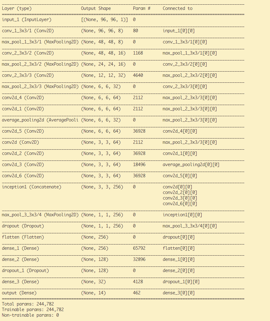
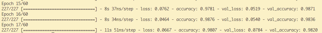
검증 데이터 기준, 2백4십만여개의 파라미터가 사용된 기존 모델의 정확도는 98.09%인 반면 24만여개로 기존에 비하여 1/10개의 파라미터를 사용한 위 모델은 98.71%의 정확도를 보였다.

안드로이드 환경에서 해당 모델을 실행시키기 위해서는 .h5 확장자를 .tflite로 변환해주어야 하는데, 변환하는 코드는 아래와 같다.

converter = tf.lite.TFLiteConverter.from_keras_model("모델경로/모델이름.h5")
tflite_model = converter.convert()

with open("./모델이름.tflite", 'wb') as f:
    f.write(tflite_model)