Multi-armed bandit problem - (2) coding

전편에 이어 multi-armed bandit을 Python으로 구현해보자.

알고리즘은 greedy, $\epsilon$-greedy, optimistic initial value 세 가지가 있었는데, greedy가 기본형이고 나머지 둘은 greedy의 단점을 보완하는 개념이었다. 따라서 전략은 greedy로 일단 정식화.

$A_{t} \doteq \underset{a}{argmax} \;\ Q_{t}(a)$

즉 $t$ 시점에서 선택하는 행동 $A$이란 기댓값 $Q_{t}(a)$를 최대화 하는 행동이어야 하고, 기댓값을 근사시켜야 할 $q_{*}(a)$가 존재하나 우리는 $q_{*}(a)$를 모르는 상태다.

다만, 이번에는 실습을 위해 $q_{*}(a)$를 랜덤으로 생성해서 알고리즘으로 찾은 $Q_{t}(a)$와 비교해보도록 하자.

위와 같이 정의된 환경을 구현하려면 numpy를 써서 난수를 발생시키고 matplolib으로 시각화도 시켜볼 수 있다.

import numpy as np
import matplotlib as plt
np.random.seed(seed=777)
qStras = np.random.normal(0, 0.8, 10)
aOpt = qStras.argmax()
aOpt

일단 위와 같이 np.random.normal(loc, scale, size) 함수를 이용해 평균 0, 표준편차 0.8, 표본사이즈 10의 난수들을 생성했다. 그리고 실습의 재현성을 위해 난수 시드를 777로 추가해줬으나 삭제하거나 다른 시드로 바꿔도 무방하다.

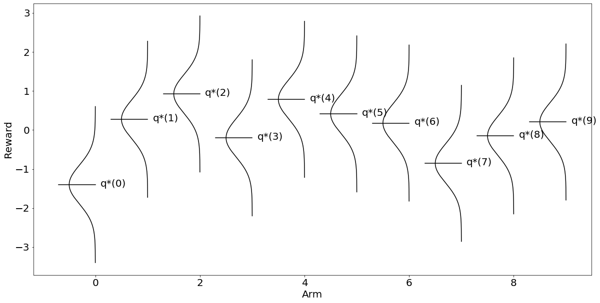
이 경우 $t$ 시점에서 최적 $a$를 출력해보면 9라고 뜰 것이다(aOpt). 즉 열번째 bandit의 레버를 당기는 행동이 최적이란 건데, 그래프로 출력해보면 더욱 직관적으로 알 수 있다.

아래는 교수님이 알려준 시각화 코드다. 어차피 다른 방식으로 시각화해도 되고 line별 의미는 알고리즘 학습 관점에서 덜 중요해 보인다. 데이터 시각화 수업이면 중요하겠지만 여기서는 ypos로 qStars[each]를 받는다는 것 정도가 포인트.

plt.rcParams["figure.figsize"] = (20,10)
plt.rcParams.update({'font.size': 20})

def draw_gaussian_at(support, sd=1.0, height=1.0, 
        xpos=0.0, ypos=0.0, ax=None, **kwargs):
    if ax is None:
        ax = plt.gca()
    gaussian = np.exp((-support ** 2.0) / (2 * sd ** 2.0))
    gaussian /= gaussian.max()
    gaussian *= height
    ax.plot(gaussian + xpos, support + ypos, **kwargs)
    ax.plot([xpos-0.7,xpos], [ypos]*2, **kwargs)
    ax.annotate('q*('+str(xpos)+')', (xpos+0.1, ypos-0.05))
    

support = np.linspace(-2, 2, 1000)
fig, ax = plt.subplots()
for each in range(10):
    draw_gaussian_at(support, sd=0.5, height=-0.5, xpos=each, ypos=qStars[each], ax=ax, color='k')
    
ax.set_xlabel('Arm')
ax.set_ylabel('Reward')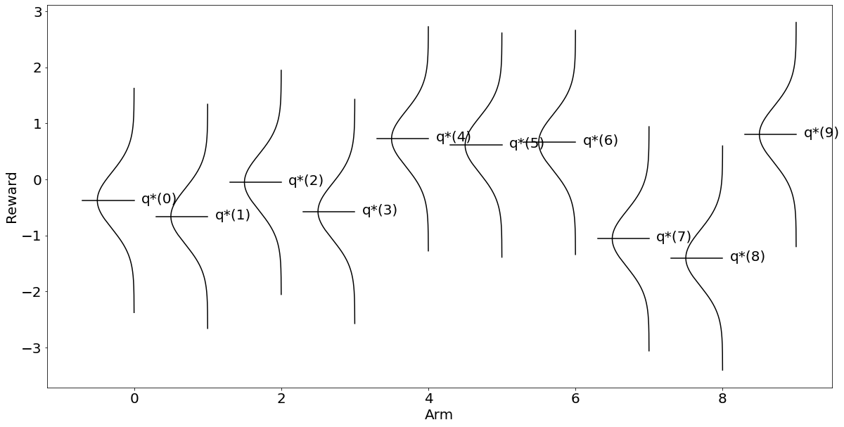

위와 같이 직관적으로 보상은 $q_{*}(9)$이 가장 크다는 것을 알 수 있다. 그럼 알고리즘을 사용해도 근사적 결과를 얻을 수 있을까?

전편에서 $\epsilon$-greedy 전략은 1-$\epsilon$ 확률로 greedy하게 exploitation을 하고, $\epsilon$ 확률로 exploration을 해보자는 아이디어였다.

$\begin{cases} A_{t}=\underset{a}{armax} \;\ Q_{t}(a), with \;\ prob \;\ 1-\epsilon \\others, \;\ with \;\ prob \;\ \epsilon \end{cases}$

따라서 딕셔너리 형태로 bandit 번호와 행위의 범위를 지정할 때 $\epsilon$도 같이 (0, 1) 범위로 지정해준다. 다만 여기서는 일단 exploration을 안 하고 exploitation만 한다는 가정 하에 eps를 0으로 줘봤다.

A = np.arange(len(qStars))
n_a = {a:0 for a in A}
Q_a = {a:0 for a in A}
eps = 0

다음으로 지정한 범위 내에서 시행이 계속 돌아야 하므로 $\epsilon$-greedy 전략에 맞게 순환 루프를 정의해준다. 시행은 range(10)으로 10번만 해본다.

for i in range(10):
  if np.random.random() > eps:
    a = max(Q_a, key=Q_a.get)
  else:
    a = np.random.randint(10)
  n_a[a] += 1
  R = np.random.normal(qStars[a], 0.5)
  Q_a[a] = Q_a[a] + (1/n_a[a])*(R-Q_a[a])
Q_a

위와 같이 np.randon.random() 함수를 사용해 (0, 1) 범위 내 무작위 확률을 생성해 값이 eps보다 크면 exploitation을 하고 아니면 exploration을 하도록 정의했다.

그러나 어차피 eps를 0으로 줬기에 일단 exploitation만 돌 것이다. 역시나 앞서 구한 $q_{*}(9)$가 아닌 $Q_{4}(a)$가 최적이라고 잘못 알아냈음을 확인할 수 있다.

{0: -0.30305106157668443,
 1: -0.23687505775369294,
 2: -0.43700636640913726,
 3: -0.749230797683209,
 4: 1.304876431892759,
 5: 0,
 6: 0,
 7: 0,
 8: 0,
 9: 0}

그래프로 그려도 마찬가지인데, 주의할 점은 여기서는 ax.annotate를 Q로 바꾸고 ypos로 qStars[each]가 아닌 Q_a[each]를 받는다는 점이다.

plt.rcParams["figure.figsize"] = (20,10)
plt.rcParams.update({'font.size': 20})

def draw_gaussian_at(support, sd=1.0, height=1.0, 
        xpos=0.0, ypos=0.0, ax=None, **kwargs):
    if ax is None:
        ax = plt.gca()
    gaussian = np.exp((-support ** 2.0) / (2 * sd ** 2.0))
    gaussian /= gaussian.max()
    gaussian *= height
    ax.plot(gaussian + xpos, support + ypos, **kwargs)
    ax.plot([xpos-0.7,xpos], [ypos]*2, **kwargs)
    ax.annotate('q*('+str(xpos)+')', (xpos+0.1, ypos-0.05))
    

support = np.linspace(-2, 2, 1000)
fig, ax = plt.subplots()
for each in range(10):
    draw_gaussian_at(support, sd=0.5, height=-0.5, xpos=each, ypos=Q_a[each], ax=ax, color='k')
    
ax.set_xlabel('Arm')
ax.set_ylabel('Reward'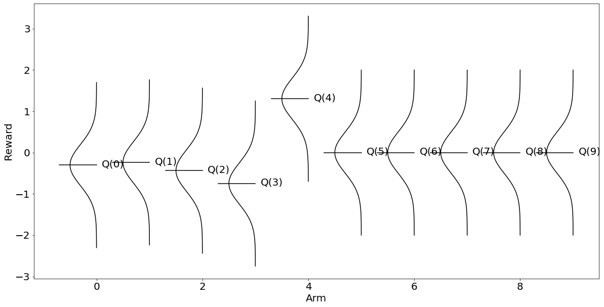

이렇게 exploitation만으로 $q_{*}(a)$를 추정해서는 역시 오류에 빠질 것이다. 따라서 eps를 0.4 정도 줘서 exploration도 해본다.

A = np.arange(len(qStars))
n_a = {a:0 for a in A}
Q_a = {a:0 for a in A}
eps = 0.4

for i in range(10):
  if np.random.random() > eps:
    a = max(Q_a, key=Q_a.get)
  else:
    a = np.random.randint(10)
  n_a[a] += 1
  R = np.random.normal(qStars[a], 0.5)
  Q_a[a] = Q_a[a] + (1/n_a[a])*(R-Q_a[a])
Q_a

이때 np.random.randit(10)은 0부터 9까지 임의의 정수를 반환해 exploration에 취할 행위를 선택한다는 의미다. 이렇게 exploration을 좀 해보면 흥미롭게도 열번째 bandit을 당기는 행위의 기댓값을 약 0.71로 가장 높게 추정함으로써 답안에 해당하는 $q_{*}(9)$을 찾았음을 알 수 있다.

{0: -0.22418027673786103,
 1: -0.6922404727061542,
 2: -0.3105419526656048,
 3: -1.3396832293777265,
 4: 0,
 5: 0,
 6: 0,
 7: 0,
 8: 0,
 9: 0.709322234273151}

plt.rcParams["figure.figsize"] = (20,10)
plt.rcParams.update({'font.size': 20})

def draw_gaussian_at(support, sd=1.0, height=1.0, 
        xpos=0.0, ypos=0.0, ax=None, **kwargs):
    if ax is None:
        ax = plt.gca()
    gaussian = np.exp((-support ** 2.0) / (2 * sd ** 2.0))
    gaussian /= gaussian.max()
    gaussian *= height
    ax.plot(gaussian + xpos, support + ypos, **kwargs)
    ax.plot([xpos-0.7,xpos], [ypos]*2, **kwargs)
    ax.annotate('Q('+str(xpos)+')', (xpos+0.1, ypos-0.05))
    

support = np.linspace(-2, 2, 1000)
fig, ax = plt.subplots()
for each in range(10):
    draw_gaussian_at(support, sd=0.5, height=-0.5, xpos=each, ypos=Q_a[each], ax=ax, color='k')
    
ax.set_xlabel('Arm')
ax.set_ylabel('Reward')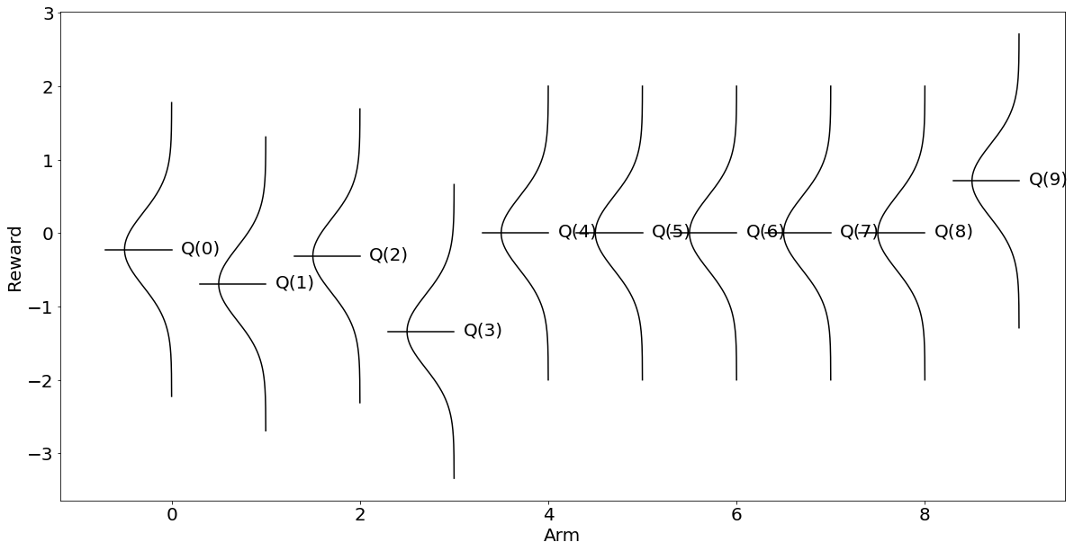

그러나 다른 사람이 이 코드를 따라했을 때 eps를 0.4로 늘렸다고, 나처럼 한 번에 정확한 $q_{*}(a)$를 찾아내진 못할 수도 있다. 왜냐하면 확률적으로 exploration을 할 행위를 선택하기 때문이다.

따라서 모두가 정확한 추정에 수렴하려면 eps를 올려주거나 시행 횟수를 늘리거나 혹은 둘 다 올려줘야 한다. eps를 0.5, 시행 횟수를 1000으로 늘려봤다. 만약 이것이 비즈니스의 문제라면 기업에게 비용의 증가를 의미한다.

A = np.arange(len(qStars))
n_a = {a:0 for a in A}
Q_a = {a:0 for a in A}
eps = 0.5

for i in range(1000):
  if np.random.random() > eps:
    a = max(Q_a, key=Q_a.get)
  else:
    a = np.random.randint(10)
  n_a[a] += 1
  R = np.random.normal(qStars[a], 0.5)
  Q_a[a] = Q_a[a] + (1/n_a[a])*(R-Q_a[a])
Q_a

{0: -0.4029929400985527,
 1: -0.746106470022782,
 2: -0.0013862506773358076,
 3: -0.5808114538588991,
 4: 0.7314208889115313,
 5: 0.6147862350262175,
 6: 0.6097090780444144,
 7: -1.0353344864044787,
 8: -1.3115024659861823,
 9: 0.7877542879459445}

plt.rcParams["figure.figsize"] = (20,10)
plt.rcParams.update({'font.size': 20})

def draw_gaussian_at(support, sd=1.0, height=1.0, 
        xpos=0.0, ypos=0.0, ax=None, **kwargs):
    if ax is None:
        ax = plt.gca()
    gaussian = np.exp((-support ** 2.0) / (2 * sd ** 2.0))
    gaussian /= gaussian.max()
    gaussian *= height
    ax.plot(gaussian + xpos, support + ypos, **kwargs)
    ax.plot([xpos-0.7,xpos], [ypos]*2, **kwargs)
    ax.annotate('Q('+str(xpos)+')', (xpos+0.1, ypos-0.05))
    

support = np.linspace(-2, 2, 1000)
fig, ax = plt.subplots()
for each in range(10):
    draw_gaussian_at(support, sd=0.5, height=-0.5, xpos=each, ypos=Q_a[each], ax=ax, color='k')
    
ax.set_xlabel('Arm')
ax.set_ylabel('Reward')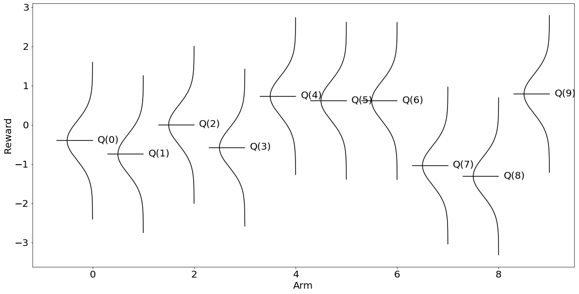

위와 같이 알고리즘이 찾아낸 결과와 답안인 $q_{*}(9)$가 일치함을 알 수 있다. 이것은 처음 시각화한 $q_{*}(a)$의 보상 그래프와 형태를 거의 구분하기 어렵다.

결국, bandit 여러 개를 존나 당겨보면서 탐색하면 언젠가는 가장 보상을 잘 주는 것을 찾을 수 있다는 이야기다.

그러나 일반적으로 우리의 자원은 유한하기에 좀 더 개꿀 빨 수 있는 방법을 찾아야 하고 강화학습은 그것을 목적으로 한다.

참고: SUTTON, Richard S.; BARTO, Andrew G. Reinforcement learning: An introduction. MIT press, 2018.
사사: 숭실대학교 산업정보시스템공학과 강창묵 교수님.