교차 검증의 정확도를 알 수 있는 함수의 종류는 다음과 같다.
- accuracy_score
- precision_score
- recall_score
- cross_val_score
- cross_validate
- KFold
- StratifiedKFold
- LeaveOneOut
- LeavePOut
- ShuffleSplit
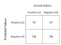
분류 모델의 예측 결과와 실제값을 비교하여 행렬 형태로 나타낸 것을 Confusion Matrix(혼동 행렬)이라고 한다. 이는 분류 모델의 성능 평가 지표가 되며 최적화에 중요한 역할을 한다.
📌 Confusion Matrix
Confusion Matrix는 다음과 같이 4개의 값으로 구성된다.
- True Positive (TP) : 모델이 positive로 예측한 것 중 실제 positive인 경우
- False Positive (FP) : 모델이 positive로 예측한 것 중 실제 negative인 경우
- False Negative (FN) : 모델이 negative로 예측한 것 중 실제 positive인 경우
- True Negative (TN) : 모델이 negative로 예측한 것 중 실제 negative인 경우
Confusion Matrix를 바탕으로 다양한 분류 성능 평가 지표를 계산할 수 있다. 그 중에서 가장 많이 사용되는 평가 지표는 정확도, 정밀도, 재현율, F1 score, AUC, ROC curve 등이 있다.
📌 정확도 (accuracy)
- 정확도가 높다고 해서 항상 올바른 모델은 아니다.
- 정확도는 분류 모델의 예측 결과와 실제 결과가 얼마나 일치하는지를 나타내는 지표이다.
from sklearn.metrics import accuracy_score
accuracy = accuraycy_score(y_true, y_pred)
print('Accuracy:', accuracy)
📌 정밀도와 재현율은 어떤 상황에서 중요한 지표로서 선택될 것인가?
1. 정밀도 (precision)
- 실제 값이 Negative일 때, Positive로 잘못 판단하게 되면 생기는 경우이다.
- 예를 들어, 스팸 메일 분류 시 스팸 메일인 것을 스팸 메일이 아닌 일반 메일로 분류하는 경우이다.
from sklearn.metrics import precision_score
precision = precision_score(y_true, y_pred)
print('Precision:', precision)
2. 재현율 (recall)
- 실제 값이 Positive일 때, Negative로 잘못 판단하게 되면 생기는 경우이다.
- 예를 들어, 암환자 분류 시 양성인 암환자를 음성으로 잘못 판단하게 되는 경우이다.
from sklearn.metrics import recall_score
recall = recall_score(y_true, y_pred)
print('Recall:', recall)
📌 정밀도와 재현율의 trade-off 관계
- 정밀도, 재현율은 특정 레이블 (0 또는 1)에 속하는지 계산하기 위해 label 결정 확률을 구하는 것이다.
- sklearn에서 정밀도와 재현율은 trade-off 관계이다. 즉, 한 쪽이 높아지면 한 쪽이 낮아지는 반비례 관계이다.
- 이진 분류 임계값 조절시에는 binarizer(threshold=값)으로 조정이 가능하다.
참고) Binarizer
sklearn.preprocessing.Binarizer(*, threshold=0.0, copy=True)- 데이터를 0 또는 1로 이진화할 시에 Binarize()함수는 임계값 보다 큰 값은 1, 작은 값은 0에 mapping된다.
- threshold parameter를 통해 임계값을 지정하며 0.0이 default이다.
- copy parameter는 True가 default이다. 만약 False로 지정한다면 원본 데이터(array)자체가 이항변수화 변환 후의 값으로 교체되어버린다.
binarizer = Binarizer(threshold=2.0)
In[9]: x = array([[10,-10,1], [5.0.2], [0,10,3]])
In[10]: binaizer.transform(X)
- 코드 실행 시 threshold가 default값인 0.0에서 2.0으로 지정되었으므로 결과는 다음과 같이 된다. ```python out[10]: array([[1,0,0], [1.0.0], [0,1,1]])
📌 F1 score
- F1 score: 정밀도, 재현율을 결합한 조화 평균이다. 따라서 데이터 label이 균형적이지 못할 때 모델의 성능을 정확하게 평가할 수 있는 지표이다.
- F1 = (2* (precision x recall) / (precision+recall))
- precision = 0.5, recall = 0.5일 때 f1 score이 precision = 0.9, recall = 0.1일 때보다 f1 score이 높게 나온다.
아래와 같이 f1 score를 함수로 나타내거나 sklearn package의 함수를 사용할 수 있다.
from sklearn.metrics import f1_score
📌 ROC curve(Receiver Operation Characterstic Curve), AUC
- ROC curve는 이진 분류 예측 시 사용한다. FPR이 변할 때 TPR이 어떻게 변하는지 나타내는 고선이다. 즉, FPR의 변화율에 따른 TPR의 변화 곡선이다. 이를 그래프 상에 그리면, FPR이 x축, TPR이 y축에 온다.
- ROC curve 자체는 FPR, TPR 변화의 값을 볼 때 사용하고 분류의 성능 지표로 사용하는 것은 ROC curve 면적에 기반한 AUC값이다. ROC curve 면적이 밑이 넓고, 1에 가까울 수록 좋은 수치이다. (-> FPR이 작고 TPR이 클 수록 가능하다.)
import numpy as np
import matplotlib.pyplot as plt
from sklearn.metrics import roc_curve, auc

# 모델 예측 결과와 실제 결과가 있는 리스트를 생성
y_pred = [0.1, 0.3, 0.5, 0.2, 0.7, 0.8, 0.4, 0.9, 0.6, 0.7]
y_true = [0, 1, 1, 0, 1, 1, 0, 1, 0, 1]

# fpr, tpr, thresholds 계산
fpr, tpr, thresholds = roc_curve(y_true, y_pred)

# AUC 계산
roc_auc = auc(fpr, tpr)

# ROC Curve 그리기
plt.figure(figsize=(8,8))
plt.plot(fpr, tpr, color='darkorange', lw=2, label='ROC curve (area = %0.2f)' % roc_auc)
plt.plot([0, 1], [0, 1], color='navy', lw=2, linestyle='--')
plt.xlabel('False Positive Rate')
plt.ylabel('True Positive Rate')
plt.title('Receiver Operating Characteristic Curve')
plt.legend(loc="lower right")
plt.show()
