
데이터 마이닝
-
기계학습 (Machine Learning) : 컴퓨터가 데이터간의 관계를 학습하여, 새로운 수식(Model)을 도출하는 작업
-
기계학습의 핵심 Point :
- 학습 능력 : 컴퓨터가 데이터를 얼마나 잘 학습하여 Model을 도출하는가
- 일반화 능력 : 새로운 데이터가 들어왔을 때, 얼마나 잘 예측/대응하는가
-
기계학습의 3요소:
- 데이터(교과서) : 학습의 목저겡 맞게 데이터를 깔끔하게 다듬는 작업이 필요
- 특성 공학 (Feature Engineering)
- 알고리즘(선생님) : 학습의 목적과 데이터의 특성에 맞게 선택
- 선형회귀 / 결정나무 / 앙상블 / 딥러닝 ...
- 하드웨어(학생)
- CPU / GPU / ...
- 비용
- 필요한 라이브러리 불러오기
import pandas as pd
import matplotlib as mpl
import plotly.express as px
import scipy.stats as stats
import numpy as np

mpl.rc('font', family = 'AppleGothic')

df1 = pd.read_csv('01_Data.csv')
기계학습의 종류
1. 지도 학습(Supervised Learning) : 목표변수(Y)와 설명변수(X)의 관계를 학습해서, 새로운 X가 들어올 때, Y를 예측/분류
- 회귀 (Regression - Y 연속형) : 특정 값을 최대한 가깝게 예측하는 것이 목적
- 분류 (Classification - Y 범주형) : 특정 항목인지 아닌지를 정확하게 분류하는 것이 목적(평가 지표들이 많다!)
- Ex) 고객 해약 예측 (정상 / 해악) / 스팸메세지 분류기 (스팸/정상) / 주가 예측 (회사의 정보 -> 주가) ...
2. 비지도학습(Unsupervised Learning) : 설명변수(X) 데이터 간의 수학적 거리/ 유사성 / 상관성 등을 이용하여, 비슷한 유형의 데이터를 묶거나 연관있는 데이터를 찾거나, 데이터의 차원을 줄이는 등의 학습 기법
- 군집분석 (Clustering) : 비슷한 위치 또는 가가운 위치의 (특성이 비슷한) 데이터를 묶어주는 학습 기법
- 차원축소 : 특정 데이터의 항목 수 (Columns)를 줄이는 기법
- 연관분석 : 특정 데이터의 유사한 항목을 찾아주는 기법
Ex) 장바구니 분석 / 추천 시스템 ...
- 준지도 학습 (Semi Supervised learning) : 비지도학습 + 지도학습 결합
3. 강화학습(Reinforcement Learning) : 컴퓨터 시뮬레이션을 통해 사용자가 설정한 환경에 대해, 적절한 보상이 주어지는 방향으로 학습을 수행
- 데이터가 없이도 학습이 가능
- 게임 AI (알파고)
지도 학습 절차
1. 데이터 핸들링 (데이터를 병합 / 파생 변수 생성 / 데이터 선택 / 이상치 제거 /...)
2. 학습의 목표변수(Y)와 설명변수(X)를 설정
- 유의 사항 : 사용되는 X 설명변수는 새로 들어올 데이터에 대한 값으로 설정
3. 학습 데이터(Train Set)와 검증 데이터(Test Set)를 분할
- 검증 데이터(Test Set)는 절대로 학습에 참여하지 않는다!
- (교차검증 기법에서 Validation Set은 학습에 참여함 <-> Test Set과 별개!)
4. 학습 수행
- 특성공학 (Feature Engineering) : 학습에 맞게 데이터를 처리
- 스케일링 / 인코딩 / 교차검증 / 변수선택법 ...
- 학습
5. 학습 된 모델의 성능을 평가
- 학습 능력
- 일반화 능력
6. 적용(새로운 데이터 입력 / 파일형태로 저장)
- 고객들의 정보를 이용하여, 해약 여부를 판별하는 모델을 생성
1. 데이터 핸들링
✔︎ 'State' 컬럼의 unique 값 확인하기
df1['State'].unique()
>> array(['계약확정', '기간만료', '해약확정', '해약진행중'], dtype=object)
✔︎ 'State'컬럼을 매핑하여 '해약여부' 파생변수 생성
df1['해약여부'] = df1['State'].replace({'계약확정':0, '기간만료':1,
                                   '해약확정':1, '해약진행중':1})
df1['해약여부'].value_counts()
>> 해약여부
0    50620
1      681
Name: count, dtype: int64
✔︎ 결측치 제거 (Y값에는 결측치가 있으면 안됨)
df2 = df1.dropna()2. 목표변수 Y / 설명변수 X 선택
Y = df2['해약여부']
X = df2[['Age', 'Credit_Rank', 'Amount_Month', 'Term']]
3. 학습 데이터와 검증 데이터를 분할
from sklearn.model_selection import train_test_split- random state를 통해서 계속 같은 test set을 얻을 수 있음
X_train, X_test, Y_train, Y_test = train_test_split(X,Y,
                                                   random_state = 1234)
4. 학습을 수행
from sklearn.tree import DecisionTreeClassifiermodel = DecisionTreeClassifier()
model.fit(X_train, Y_train)
>> DecisionTreeClassifier()
In a Jupyter environment, please rerun this cell to show the HTML representation or trust the notebook.
On GitHub, the HTML representation is unable to render, please try loading this page with nbviewer.org.5. 평가 수행 (학습능력 / 일반화능력)
- 기존에 사용한 X 데이터를 이용해 예측값을 계산
Y_train_pred = model.predict(X_train)
Y_test_pred = model.predict(X_test)- 정확도 평가 지표 불러오기
from sklearn.metrics import accuracy_score✔︎ 학습 능력 평가
accuracy_score(Y_train, Y_train_pred)✔︎ 일반화 능력 평가
accuracy_score(Y_test, Y_test_pred)6. 적용
x1 = input('고객 연령을 입력하시오 : ')
x2 = input('고객 신용 등급을 입력하시오 : ')
x3 = input('계약할 월 랜탈비용을 입력하시오 : ')
x4 = input('계약할 기간을 입력하시오 : ')

>> 고객 연령을 입력하시오 : 29
고객 신용 등급을 입력하시오 : 3
계약할 월 랜탈비용을 입력하시오 : 100000
계약할 기간을 입력하시오 : 12
✔︎ 해약 : 1 / 정상 : 0
input_data = pd.DataFrame([[x1,x2,x3,x4]], columns=X.columns)
model.predict(input_data)
✔︎ 생성된 모델을 파일 형태로 저장
- 파이썬에 있는 객체나 변수를 파일형태로 저장
import picklepickle.dump(model, open('model.sav', 'wb'))모델평가
- 분류모델에서의 평가
- 정확도 (Accuracy) = 예측 결과가 동일한 데이터의 수 / 전체 예측 데이터의 수
- 클래스(나누고자 하는 항목)의 비율이 균형을 이룰 때 주로 사용
- 모든 클래스가 동등한 중요도를 가지며, 비율도 같을 때
- 단순 이진분류에서 데이터의 비율이 깨져있는 경우 (Imbalanced Data) 모델의 성능이 잘못 측정됨
- 오차 행렬 (Confusion Matrix)
- 정상 (Negative)을 정상으로 해약(Positive)을 해약으로 분류하는 데이터의 수를 표로 정리
- 정밀도 (Precision) : True Positive / (False Positive + True Positive)
- (정확하게 해약으로 분류한 수) / (예측을 해약으로 분류한 수)
- 예측 성능을 더욱 정밀하게 측정하기 위해 사용되는 지표
- False Positive의 개수를 낮추는데에 초점 / ex) 스팸메시지 분류
- 재현율 (Recall) : True Positive / (False Negative + True Positive)
- (정확하게 해약으로 분류한 수) / (실제 해약인 데이터 수)
- Sensitivity (민감도) / TPR(True Positive Rate)
- 실제 문제가 있는 데이터를 문제가 없다고 잘못 판단할 때 발생하는 이슈를 나타내는 지표
- False Negative를 낮추는 데 초점 / ex) 암진단, 불량여부, 해약여부 ...
- 두 수치가 모두 좋아야 한다.
from sklearn.metrics import precision_score, recall_score- 0 / 1 의 이진 분류에서 1값을 Positive로 뒀을 때, 정밀도
print('학습 데이터의 Precision : ', precision_score(Y_train, Y_train_pred))
print('검증 데이터의 Precision : ', precision_score(Y_test, Y_test_pred))

>> 학습 데이터의 Precision :  0.9787234042553191
검증 데이터의 Precision : 0.0- 비율이 깨진 데이터에서 Recall을 중점으로 보는 실무적 데이터의 경우,Recall 값이 Precision에 비해 현저히 낮게 나오는 경향
print('학습 데이터의 Recall : ', recall_score(Y_train, Y_train_pred))
print('검증 데이터의 Recall : ', recall_score(Y_test, Y_test_pred))

>> 학습 데이터의 Recall :  0.11219512195121951
검증 데이터의 Recall : 0.0- 분류모델 평가 지표를 모두 확인
from sklearn.metrics import classification_report- 학습
print(classification_report(Y_train, Y_train_pred))

>>               precision    recall  f1-score   support

           0       0.99      1.00      0.99     30075
           1       0.98      0.11      0.20       410

    accuracy                           0.99     30485
   macro avg       0.98      0.56      0.60     30485
weighted avg       0.99      0.99      0.98     30485
- F1 Score : 정밀도와 재현율의 결합지표
- 정밀도와 재현율이 모두 중요한 (균형이 필요한 경우에 사용)
- 0 ~ 1
pd.DataFrame(model.predict_proba(X_test))

>>
0	1
0	0.980392	0.019608
1	1.000000	0.000000
2	1.000000	0.000000
3	1.000000	0.000000
4	1.000000	0.000000
...	...	...
10157	0.909091	0.090909
10158	0.976378	0.023622
10159	0.500000	0.500000
10160	1.000000	0.000000
10161	1.000000	0.000000
10162 rows × 2 columns- Threshold는 분류된 각 클래스 별 확률 값 중 더 큰 값으로 (0.5/ 50%) 예측을 실시
- Threshold 값을 조정해서, 판단을 다르게 수행
- '해약'으로 판단할 확률이 15% (0.15)만 넘어도 "해약"으로 예측
from sklearn.preprocessing import Binarizer- 모델 분류의 분류기준을 변경
customer_threshold = 0.15
Binarizer(threshold = customer_threshold)

>> Binarizer(threshold=0.15)
In a Jupyter environment, please rerun this cell to show the HTML representation or trust the notebook.
On GitHub, the HTML representation is unable to render, please try loading this page with nbviewer.org.- 해약으로 판단할 확률만 추출
predict_proba_col = model.predict_proba(X_test)[:, 1].reshape(-1,1)- 새로운 임계값을 적용해 예측
custom_bin = Binarizer(threshold=customer_threshold).fit(predict_proba_col)
Y_test_pred2 = custom_bin.transform(predict_proba_col) #15%를 기준으로 해약을 분류
print(classification_report(Y_test, Y_test_pred2))
>> precision recall f1-score support
0 0.99 0.98 0.98 10029
1 0.07 0.12 0.09 133
accuracy 0.97 10162
macro avg 0.53 0.55 0.54 10162
weighted avg 0.98 0.97 0.97 10162- 임계값을 변경하면 실제 F1 score 값이 증가
- 판단 기준을 변경한 것이기에, 모델의 성능은 높아졌다고 볼 수 없음
from sklearn.metrics import precision_recall_curve- 해약으로 분류할 확률만 추출
Y_test_proba1 = model.predict_proba(X_test)[:, 1]- 각 Threshold에서 계산된 Recall과 Precision 계산
precision1, recall1, threshold1 = precision_recall_curve(Y_test, Y_test_proba1)threshold1
>> array([0. , 0.00719424, 0.00735294, 0.00869565, 0.00961538,
0.01204819, 0.01219512, 0.01265823, 0.01282051, 0.01298701,
0.01315789, 0.01333333, 0.01351351, 0.01388889, 0.01428571,
0.01694915, 0.01724138, 0.01818182, 0.01851852, 0.01923077,
0.01960784, 0.02 , 0.02040816, 0.0212766 , 0.02173913,
0.02222222, 0.02362205, 0.02380952, 0.02439024, 0.025 ,
0.02542373, 0.02564103, 0.02631579, 0.02702703, 0.02777778,
0.02941176, 0.03030303, 0.03125 , 0.03225806, 0.03333333,
0.03389831, 0.03448276, 0.0375 , 0.03846154, 0.04 ,
0.04761905, 0.05 , 0.05084746, 0.05128205, 0.05263158,
0.05405405, 0.05555556, 0.05714286, 0.05882353, 0.06060606,
0.0625 , 0.06666667, 0.07692308, 0.08333333, 0.09090909,
0.09375 , 0.1 , 0.10526316, 0.11111111, 0.125 ,
0.14285714, 0.15384615, 0.16666667, 0.18181818, 0.2 ,
0.21428571, 0.22222222, 0.25 , 0.28571429, 0.3 ,
0.30769231, 0.33333333, 0.375 , 0.4 , 0.5 ,
0.66666667, 1. ])df_cm_curve = pd.DataFrame()
df_cm_curve['threshold'] = threshold1
df_cm_curve['precision'] = precision1[:-1]
df_cm_curve['recall']= recall1[:-1]- 시각화를 쉽게 하기 위해 데이터 프레임을 재구조화
p1 = df_cm_curve.melt(id_vars=['threshold'])px.line(p1, x='threshold', y='value', color='variable')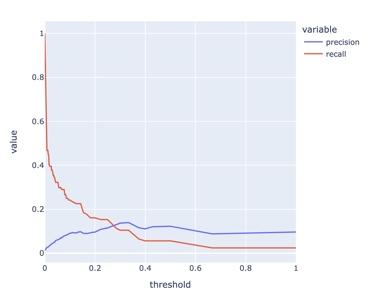
ROC Curve & AUC
- ROC (Receiver Operation Characteristic Curve)
- '수신자판단곡선'이라고 불림
- 모델에 대한 성능지표를 시각화하여 표현/의학 분야/머신러닝 이진분류 모델
- FPR(False Positive Rate)에 따라 TPR(True Positive Rate, Recall)값이 어떻게 변화하는지를 시각화한 곡선
- TPR(민감도)와 TNR(특이성 / Specificity) 대한 시각화
from sklearn.metrics import roc_curve- 해약으로 분류 될 확률값
Y_test_proba1

>> array([0.01960784, 0.        , 0.        , ..., 0.5       , 0.        ,
       0.        ])
fprs, tprs, threshold2 = roc_curve(Y_test, Y_test_proba1)df_roc = pd.DataFrame()
df_roc['FPR'] = fprs
df_roc['TPR'] = tprs
df_roc['Threshold'] = threshold2- 그래프에 세부 요소를 추가
import plotly.graph_objects as gofig1 = px.line(df_roc, x='FPR', y='TPR')
fig1.add_trace(go.Scatter(x=[0,1], y=[0,1], mode='lines'))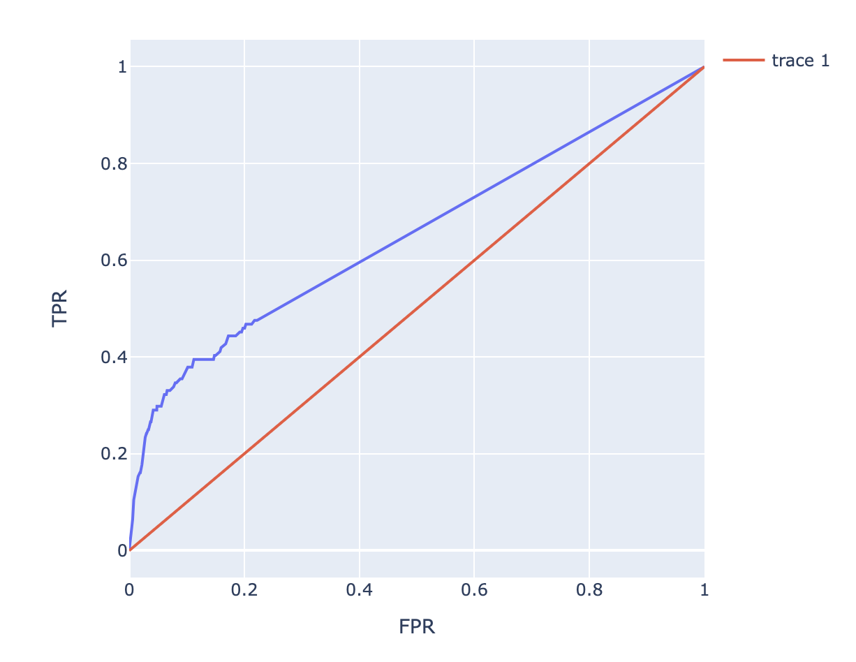
AUC (Area Under the Curve)
- ROC에서 아랫 면적을 나타내며, 이 면적은 모델의 성능을 의미
- AUC가 0.5 : 모델이 데이터를 Random하게 예측 (중앙선에 가깝게 선이 표현)
- AUC가 1.0 : 모델이 데이터를 완벽하게 예측
- AUC가 0.7이상인 경우 : 모델이 어느정도 성능을 보임
- 0.5~0.7 : 모델의 예측이 제한적이며 개선이 필요
- 실제로는 도메인마다 / 데이터마다 다름!
from sklearn.metrics import roc_auc_scoreprint('학습 AUC : ', roc_auc_score(Y_train, Y_train_pred))
print('검증 AUC : ', roc_auc_score(Y_test, Y_test_pred))
>> 학습 AUC : 0.5536660238485673
검증 AUC : 0.510552641896278회귀 모델 평가 지표
-
R^2 (결정계수) : 변동을 기반으로 예측성능을 평가하는 지표/ 회귀 모델이 데이터를 얼마나 잘 설명하고 있는가 (0 ~ 1)
-
MSE (Mean Squared Error) : 실제값과 예측값의 차이를 제곱해 평균을 계산
- 0으로 갈수록 정확한 모델
- RMS(Root Mean Square Error)
-
MAE (Mean Absolute Error) : 실제값과 예측값의 차이에 절댓값의 평균을 계산
- 0으로 갈수록 정확한 모델
Overfitting (과적합)
- 학습 데이터에 대해 성능이 월등히 높게 측정 되나 (100%) 검증 데이터에 대해 성능이 현저히 떨어지는 현상
- 컴퓨터가 학습데이터에 대해 과하게 학습을 수행 -> 일반화
- 해결 :
- 학습이 잘 수행되도록 데이터를 깔끔하게 처리
- 알고리즘을 통제 -> 특성공학(데이터를 처리 + 알고리즘 통제)
특성공학 기법을 적용하여 학습
- 특성 공학: 학습을 수행하기 위해 데이터를 깔끔하게 다듬는 과정
- 데이터마이닝에서 알고리즘의 학습 및 일반화 성능을 높이기 위한 기술
- Scaling & Encoding
- Imputation
- Cross Validation
- Hyper Parameter Tuning
- (분류) imbalanced Data Sampling
- Feature Selection
- PCA/ Clustering ...