Online Shoppers Purchasing Intention Dataset Data Set
데이터는 총 18개의 칼럼과 12330개의 rows로 구성
| Header | Description |
|---|---|
| Administrative | This is the number of pages of this type (administrative) that the user visited. |
| Administrative_Duration | This is the amount of time spent in this category of pages. |
| Informational | This is the number of pages of this type (informational) that the user visited. |
| Informational_Duration | This is the amount of time spent in this category of pages. |
| ProductRelated | This is the number of pages of this type (product related) that the user visited. |
| ProductRelated_Duration | This is the amount of time spent in this category of pages. |
| BounceRates | The percentage of visitors who enter the website through that page and exit without triggering any additional tasks. |
| ExitRates | The percentage of pageviews on the website that end at that specific page. |
| PageValues | The average value of the page averaged over the value of the target page and/or the completion of an eCommerce |
| SpecialDay | This value represents the closeness of the browsing date to special days or holidays (eg Mother's Day or Valentine's day) in |
| Month | Contains the month the pageview occurred, in string form. |
| OperatingSystems | An integer value representing the operating system that the user was on when viewing the page. |
| Browser | An integer value representing the browser that the user was using to view the page. |
| Region | An integer value representing which region the user is located in. |
| TrafficType | An integer value representing what type of traffic the user is categorized into. |
| VisitorType | A string representing whether a visitor is New Visitor, Returning Visitor, or Other. |
| Weekend | A boolean representing whether the session is on a weekend. |
| Revenue | A boolean representing whether or not the user completed the purchase. |
EDA
- 데이터를 불러오고 기본적인 정보를 보자.
library(knitr)
library(rmarkdown)
getwd()
## [1] "/Users/leehyebin/Desktop"
setwd("/Users/leehyebin/Rdata")

df <- read.csv('online_shoppers_intention.csv', stringsAsFactors = TRUE)
head(df)
##   Administrative Administrative_Duration Informational Informational_Duration
## 1              0                       0             0                      0
## 2              0                       0             0                      0
## 3              0                       0             0                      0
## 4              0                       0             0                      0
## 5              0                       0             0                      0
## 6              0                       0             0                      0
##   ProductRelated ProductRelated_Duration BounceRates ExitRates PageValues
## 1              1                0.000000  0.20000000 0.2000000          0
## 2              2               64.000000  0.00000000 0.1000000          0
## 3              1                0.000000  0.20000000 0.2000000          0
## 4              2                2.666667  0.05000000 0.1400000          0
## 5             10              627.500000  0.02000000 0.0500000          0
## 6             19              154.216667  0.01578947 0.0245614          0
##   SpecialDay Month OperatingSystems Browser Region TrafficType
## 1          0   Feb                1       1      1           1
## 2          0   Feb                2       2      1           2
## 3          0   Feb                4       1      9           3
## 4          0   Feb                3       2      2           4
## 5          0   Feb                3       3      1           4
## 6          0   Feb                2       2      1           3
##         VisitorType Weekend Revenue
## 1 Returning_Visitor   FALSE   FALSE
## 2 Returning_Visitor   FALSE   FALSE
## 3 Returning_Visitor   FALSE   FALSE
## 4 Returning_Visitor   FALSE   FALSE
## 5 Returning_Visitor    TRUE   FALSE
## 6 Returning_Visitor   FALSE   FALSE
str(df)
## 'data.frame':    12330 obs. of  18 variables:
##  $ Administrative         : int  0 0 0 0 0 0 0 1 0 0 ...
##  $ Administrative_Duration: num  0 0 0 0 0 0 0 0 0 0 ...
##  $ Informational          : int  0 0 0 0 0 0 0 0 0 0 ...
##  $ Informational_Duration : num  0 0 0 0 0 0 0 0 0 0 ...
##  $ ProductRelated         : int  1 2 1 2 10 19 1 0 2 3 ...
##  $ ProductRelated_Duration: num  0 64 0 2.67 627.5 ...
##  $ BounceRates            : num  0.2 0 0.2 0.05 0.02 ...
##  $ ExitRates              : num  0.2 0.1 0.2 0.14 0.05 ...
##  $ PageValues             : num  0 0 0 0 0 0 0 0 0 0 ...
##  $ SpecialDay             : num  0 0 0 0 0 0 0.4 0 0.8 0.4 ...
##  $ Month                  : Factor w/ 10 levels "Aug","Dec","Feb",..: 3 3 3 3 3 3 3 3 3 3 ...
##  $ OperatingSystems       : int  1 2 4 3 3 2 2 1 2 2 ...
##  $ Browser                : int  1 2 1 2 3 2 4 2 2 4 ...
##  $ Region                 : int  1 1 9 2 1 1 3 1 2 1 ...
##  $ TrafficType            : int  1 2 3 4 4 3 3 5 3 2 ...
##  $ VisitorType            : Factor w/ 3 levels "New_Visitor",..: 3 3 3 3 3 3 3 3 3 3 ...
##  $ Weekend                : logi  FALSE FALSE FALSE FALSE TRUE FALSE ...
##  $ Revenue                : logi  FALSE FALSE FALSE FALSE FALSE FALSE ...
df$Region <- as.factor(df$Region)
df$TrafficType <- as.factor(df$TrafficType)
df$Weekend <- as.factor(df$Weekend)
df$Revenue <- as.factor(df$Revenue)
df$OperatingSystems <- as.factor(df$OperatingSystems)

summary(df)
##  Administrative   Administrative_Duration Informational
##  Min.   : 0.000   Min.   :   0.00         Min.   : 0.0000
##  1st Qu.: 0.000   1st Qu.:   0.00         1st Qu.: 0.0000
##  Median : 1.000   Median :   7.50         Median : 0.0000
##  Mean   : 2.315   Mean   :  80.82         Mean   : 0.5036
##  3rd Qu.: 4.000   3rd Qu.:  93.26         3rd Qu.: 0.0000
##  Max.   :27.000   Max.   :3398.75         Max.   :24.0000
##
##  Informational_Duration ProductRelated   ProductRelated_Duration
##  Min.   :   0.00        Min.   :  0.00   Min.   :    0.0
##  1st Qu.:   0.00        1st Qu.:  7.00   1st Qu.:  184.1
##  Median :   0.00        Median : 18.00   Median :  598.9
##  Mean   :  34.47        Mean   : 31.73   Mean   : 1194.8
##  3rd Qu.:   0.00        3rd Qu.: 38.00   3rd Qu.: 1464.2
##  Max.   :2549.38        Max.   :705.00   Max.   :63973.5
##
##   BounceRates         ExitRates         PageValues        SpecialDay
##  Min.   :0.000000   Min.   :0.00000   Min.   :  0.000   Min.   :0.00000
##  1st Qu.:0.000000   1st Qu.:0.01429   1st Qu.:  0.000   1st Qu.:0.00000
##  Median :0.003112   Median :0.02516   Median :  0.000   Median :0.00000
##  Mean   :0.022191   Mean   :0.04307   Mean   :  5.889   Mean   :0.06143
##  3rd Qu.:0.016813   3rd Qu.:0.05000   3rd Qu.:  0.000   3rd Qu.:0.00000
##  Max.   :0.200000   Max.   :0.20000   Max.   :361.764   Max.   :1.00000
##
##      Month      OperatingSystems    Browser           Region      TrafficType
##  May    :3364   2      :6601     Min.   : 1.000   1      :4780   2      :3913
##  Nov    :2998   1      :2585     1st Qu.: 2.000   3      :2403   1      :2451
##  Mar    :1907   3      :2555     Median : 2.000   4      :1182   3      :2052
##  Dec    :1727   4      : 478     Mean   : 2.357   2      :1136   4      :1069
##  Oct    : 549   8      :  79     3rd Qu.: 2.000   6      : 805   13     : 738
##  Sep    : 448   6      :  19     Max.   :13.000   7      : 761   10     : 450
##  (Other):1337   (Other):  13                      (Other):1263   (Other):1657
##             VisitorType     Weekend      Revenue
##  New_Visitor      : 1694   FALSE:9462   FALSE:10422
##  Other            :   85   TRUE :2868   TRUE : 1908
##  Returning_Visitor:10551
##
##
##
##
dim(df)
## [1] 12330    18
sum(is.na(df))
## [1] 0
NA값은 없으며 결과변수 ’Revenue’가 FALSE는 10422건, TRUE가 1908건으로 불균형 데이터이다.
- Month변수의 factor순서를 보기 편하게 재배열하자.
levels(df$Month)
##  [1] "Aug"  "Dec"  "Feb"  "Jul"  "June" "Mar"  "May"  "Nov"  "Oct"  "Sep"
df$Month <- factor(df$Month, levels=levels(df$Month)[c(3, 6, 7, 5, 4, 1, 10, 9, 8, 2)])
levels(df$Month)
## [1] "Feb" "Mar" "May" "June" "Jul" "Aug" "Sep" "Oct" "Nov" "Dec"- EDA에 필요한 패키지들을 불러오자.
library(DMwR2)
## Registered S3 method overwritten by 'quantmod':
##   method            from
##   as.zoo.data.frame zoo
library(pastecs)
library(psych)
library(caret)
## Loading required package: ggplot2
##
## Attaching package: 'ggplot2'
## The following objects are masked from 'package:psych':
##
##     %+%, alpha
## Loading required package: lattice
library(ggplot2)
library(GGally)
## Registered S3 method overwritten by 'GGally':
##   method from
##   +.gg   ggplot2
library(smotefamily)
library(naniar)
library(reshape2)
library(gridExtra)
library(gapminder)
library(dplyr)
##
## Attaching package: 'dplyr'
## The following object is masked from 'package:gridExtra':
##
##     combine
## The following objects are masked from 'package:pastecs':
##
##     first, last
## The following objects are masked from 'package:stats':
##
##     filter, lag
## The following objects are masked from 'package:base':
##
##     intersect, setdiff, setequal, union
library(PerformanceAnalytics)
## Loading required package: xts
## Loading required package: zoo
##
## Attaching package: 'zoo'
## The following objects are masked from 'package:base':
##
##     as.Date, as.Date.numeric
##
## Attaching package: 'xts'
## The following objects are masked from 'package:dplyr':
##
##     first, last
## The following objects are masked from 'package:pastecs':
##
##     first, last
##
## Attaching package: 'PerformanceAnalytics'
## The following object is masked from 'package:graphics':
##
##     legend
library(FSelector)
library(Boruta)
library(ROSE)
## Loaded ROSE 0.0-4- 탐색적 분석으로 첨도 및 왜도를 알아보자.
describeBy(df[, -c(11, 12, 14, 15, 16, 17)], df$Revenue, mat = FALSE)
##
##  Descriptive statistics by group
## group: FALSE
##                         vars     n    mean      sd median trimmed    mad min
## Administrative             1 10422    2.12    3.20   0.00    1.43   0.00   0
## Administrative_Duration    2 10422   73.74  171.02   0.00   36.51   0.00   0
## Informational              3 10422    0.45    1.21   0.00    0.14   0.00   0
## Informational_Duration     4 10422   30.24  133.91   0.00    2.39   0.00   0
## ProductRelated             5 10422   28.71   40.74  16.00   20.62  17.79   0
## ProductRelated_Duration    6 10422 1069.99 1803.80 510.19  726.48 650.90   0
## BounceRates                7 10422    0.03    0.05   0.00    0.01   0.01   0
## ExitRates                  8 10422    0.05    0.05   0.03    0.04   0.02   0
## PageValues                 9 10422    1.98    9.07   0.00    0.03   0.00   0
## SpecialDay                10 10422    0.07    0.21   0.00    0.00   0.00   0
## Browser                   11 10422    2.34    1.68   2.00    1.99   0.00   1
## Revenue*                  12 10422    1.00    0.00   1.00    1.00   0.00   1
##                              max    range skew kurtosis    se
## Administrative             27.00    27.00 2.09     5.48  0.03
## Administrative_Duration  3398.75  3398.75 6.10    60.03  1.68
## Informational              24.00    24.00 4.45    33.92  0.01
## Informational_Duration   2549.38  2549.38 8.43    94.32  1.31
## ProductRelated            705.00   705.00 4.69    38.81  0.40
## ProductRelated_Duration 63973.52 63973.52 8.83   196.97 17.67
## BounceRates                 0.20     0.20 2.66     5.97  0.00
## ExitRates                   0.20     0.20 1.94     2.97  0.00
## PageValues                246.76   246.76 9.56   147.98  0.09
## SpecialDay                  1.00     1.00 3.08     8.41  0.00
## Browser                    13.00    12.00 3.24    12.82  0.02
## Revenue*                    1.00     0.00  NaN      NaN  0.00
## ------------------------------------------------------------
## group: TRUE
##                         vars    n    mean      sd  median trimmed     mad min
## Administrative             1 1908    3.39    3.73    2.00    2.78    2.97   0
## Administrative_Duration    2 1908  119.48  201.11   52.37   76.18   77.64   0
## Informational              3 1908    0.79    1.52    0.00    0.42    0.00   0
## Informational_Duration     4 1908   57.61  171.62    0.00   14.44    0.00   0
## ProductRelated             5 1908   48.21   58.27   29.00   36.26   25.20   0
## ProductRelated_Duration    6 1908 1876.21 2312.21 1109.91 1410.82 1040.40   0
## BounceRates                7 1908    0.01    0.01    0.00    0.00    0.00   0
## ExitRates                  8 1908    0.02    0.02    0.02    0.02    0.01   0
## PageValues                 9 1908   27.26   35.19   16.76   20.87   23.93   0
## SpecialDay                10 1908    0.02    0.12    0.00    0.00    0.00   0
## Browser                   11 1908    2.45    1.90    2.00    2.05    0.00   1
## Revenue*                  12 1908    2.00    0.00    2.00    2.00    0.00   2
##                              max    range skew kurtosis    se
## Administrative             26.00    26.00 1.45     2.40  0.09
## Administrative_Duration  2086.75  2086.75 3.98    23.06  4.60
## Informational              12.00    12.00 2.69     9.25  0.03
## Informational_Duration   1767.67  1767.67 4.97    31.07  3.93
## ProductRelated            534.00   534.00 3.25    15.00  1.33
## ProductRelated_Duration 27009.86 27009.86 3.33    17.65 52.93
## BounceRates                 0.20     0.20 8.26   109.82  0.00
## ExitRates                   0.20     0.20 3.47    25.84  0.00
## PageValues                361.76   361.76 3.25    17.85  0.81
## SpecialDay                  1.00     1.00 5.78    34.37  0.00
## Browser                    13.00    12.00 3.18    11.72  0.04
## Revenue*                    2.00     0.00  NaN      NaN  0.00
FALSE그룹의 Administrative_Duration, Informational, Informational_Duration, ProductRelated, ProductRelated_Duration, PageValues변수의 첨도가 모두 30이상으로 굉장히 뾰족한 분포를 보일 것으로 예상된다. 또한 모든 수치형 변수의 왜도가 0보다 큰 양수로 왼쪽으로 치우친 분포를 보일 것으로 예상된다.
TRUE그룹을 보면 Informational_Duration, BounceRates, SpecialDay변수만 30이 넘는 첨도를 보여 FALSE그룹과 차이나는 분포를 보이고 있음을 알 수 있다. TRUE그룹의 왜도 또한 모두 0보다 큰 양수로 왼쪽으로 치우친 분포를 보인다.
- 그래프로 변수별 분포를 확인해보자.
– 수치형 변수와 팩터형 변수를 따로 확인해보자.
– 우선 수치형 변수의 분포를 2번에 걸쳐서 확인해보자.
ggpairs(df, columns = c(1, 2, 3, 4, 5, 6), aes(colour = Revenue, alpha = 0.4))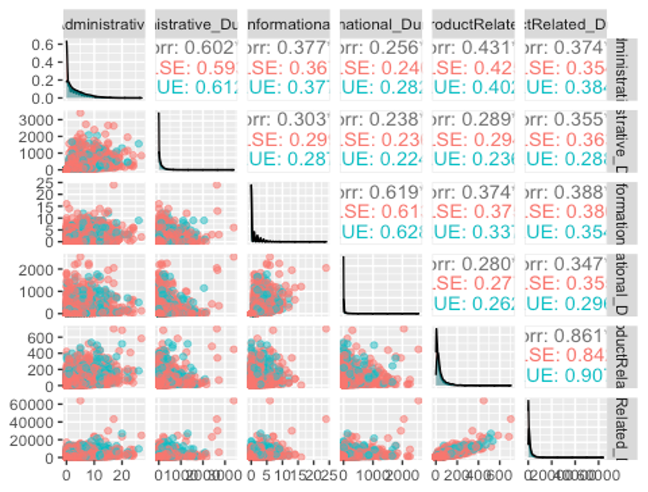
위에서 보았듯이 모든 변수가 왼쪽으로 치우친 분포를 보이고 있고, Administrative_Duration, Informational, ProductRelated, ProductRelated_Duration변수는 FALSE그룹이 TRUE그룹보다 훨씬 뾰족한 분포를 보이고 있다.
- 나머지 수치형 변수들의 분포를 그려보자.
ggpairs(df, columns = c(7, 8, 9, 10, 13), aes(colour = Revenue, alpha = 0.4))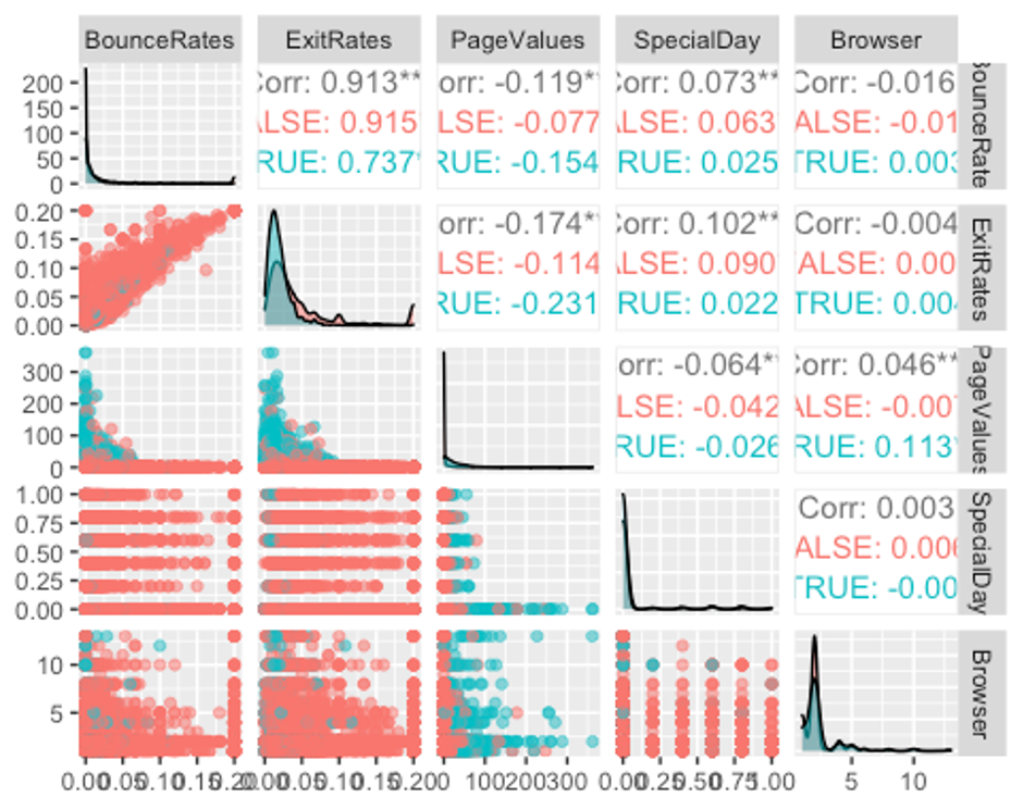
역시 모든 변수가 왼쪽으로 치우친 분포를 보이고 있으며, BounceRates, ExitRates, SpecialDay변수는 FALSE그룹보다 TRUE그룹이 뾰족한 분포를 보이고 있다.
- 다음으로 factor형 변수가 어떤 분포를 보이고 있는지 보자.
ggpairs(df, columns = c(11, 12, 14, 16, 17), aes(colour = Revenue, alpha = 0.4))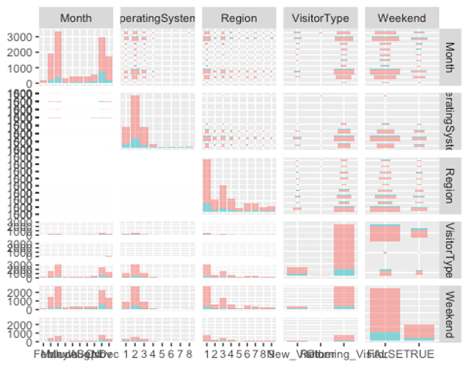
Month변수의 분포를 보면 구매 사실(Revenue변수에서 TRUE그룹)이 11월에 가장 높고, 2월에 가장 낮은 것으로 보인다. 단순한 홈페이지 방문자 수는 5월에 가장 높았다. 이는 월별 이벤트(5월의 Mother’s Day, 11월의 추수감사절, 12월의 크리스마스 등)가 홈페이지 방문자 수와 구매 여부에 상관관계가 있음을 암시한다.
Region변수의 분포를 보면 1지역에서 홈페이지 방문자수도 가장 많고, 구매도 가장 많다. VisitorType변수의 분포는 신규 고객보다 재방문 고객이 5배 이상 많았다. 또한 주말보다 평일에 홈페이지를 더 많이 방문하고 구매하는 것으로 보인다.
- 이제 수치형 변수에 이상치가 있는지 확인해보자.
– 데이터의 범위가 변수별로 차이 나므로 평균이 0, 분산이 1이 되도록 스케일링 하고 데이터를 wide형식에서 long형식으로 바꿔주자.
df_numeric <- df[, c(1, 2, 3, 4, 5, 6, 7, 8, 9, 10, 13, 18)]
model_scale <- preProcess(df_numeric, method = c('center', 'scale'))
scaled_df <- predict(model_scale, df_numeric)
melt_df <- melt(scaled_df, id.vars = 'Revenue')
head(melt_df)
##   Revenue       variable      value
## 1   FALSE Administrative -0.6969647
## 2   FALSE Administrative -0.6969647
## 3   FALSE Administrative -0.6969647
## 4   FALSE Administrative -0.6969647
## 5   FALSE Administrative -0.6969647
## 6   FALSE Administrative -0.6969647
p1 <- ggplot(melt_df, aes(x = variable, y = value, fill = Revenue)) + geom_boxplot()
p1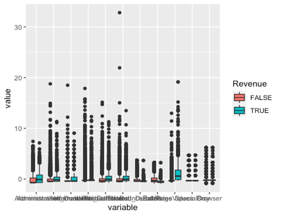
모든 수치형 변수에 이상치가 있다.
- 사분위수 99% 범위 밖의 이상치는 75% 사분위수로 바꿔주고, 1%내의 이상치는 25% 사분위수로 바꿔준다.
outHigh <- function(x){
  x[x > quantile(x, 0.99)] <- quantile(x, 0.75)
  x
}

outLow <- function(x){
  x[x < quantile(x, 0.01)] <- quantile(x, 0.25)
  x
}

df_2 <- data.frame(lapply(df[, -c(11, 12, 14, 15, 16, 17, 18)], outHigh))
df_2 <- data.frame(lapply(df_2, outLow))
df_2$Month <- df$Month
df_2$OperatingSystems <- df$OperatingSystems
df_2$Region <- df$Region
df_2$TrafficType <- df$TrafficType
df_2$VisitorType <- df$VisitorType
df_2$Weekend <- df$Weekend
df_2$Revenue <- df$Revenue- 이상치 변경 후의 boxplot을 다시 그려보자.
df_numeric2 <- df_2[, -c(12:17)]
model_scale2 <- preProcess(df_numeric2, method = c('center', 'scale'))
scaled_df2 <- predict(model_scale2, df_numeric2)
melt_df2 <- melt(scaled_df2, id.vars = 'Revenue')
head(melt_df2)
##   Revenue       variable      value
## 1   FALSE Administrative -0.7336044
## 2   FALSE Administrative -0.7336044
## 3   FALSE Administrative -0.7336044
## 4   FALSE Administrative -0.7336044
## 5   FALSE Administrative -0.7336044
## 6   FALSE Administrative -0.7336044
p2 <- ggplot(melt_df2, aes(x = variable, y = value, fill = Revenue)) + geom_boxplot()
p2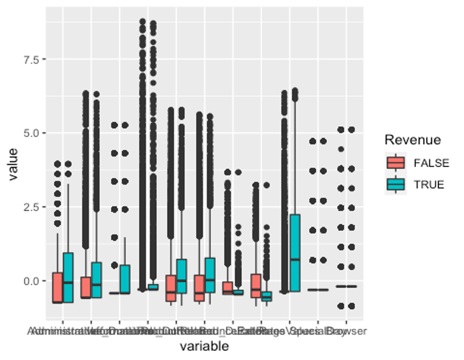
잘 변경된 것으로 보인다.
- 변수들의 상관관계를 확인하자.
str(df_numeric2)
## 'data.frame':    12330 obs. of  12 variables:
##  $ Administrative         : num  0 0 0 0 0 0 0 1 0 0 ...
##  $ Administrative_Duration: num  0 0 0 0 0 0 0 0 0 0 ...
##  $ Informational          : num  0 0 0 0 0 0 0 0 0 0 ...
##  $ Informational_Duration : num  0 0 0 0 0 0 0 0 0 0 ...
##  $ ProductRelated         : num  1 2 1 2 10 19 1 7 2 3 ...
##  $ ProductRelated_Duration: num  0 64 0 2.67 627.5 ...
##  $ BounceRates            : num  0.2 0 0.2 0.05 0.02 ...
##  $ ExitRates              : num  0.2 0.1 0.2 0.14 0.05 ...
##  $ PageValues             : num  0 0 0 0 0 0 0 0 0 0 ...
##  $ SpecialDay             : num  0 0 0 0 0 0 0.4 0 0.8 0.4 ...
##  $ Browser                : num  1 2 1 2 3 2 4 2 2 4 ...
##  $ Revenue                : Factor w/ 2 levels "FALSE","TRUE": 1 1 1 1 1 1 1 1 1 1 ...
df_numeric2 <- df_numeric2[, -12]
cor_df <- cor(df_numeric2)
chart.Correlation(df_numeric2, histogram = TRUE, pch = 19, method = 'pearson')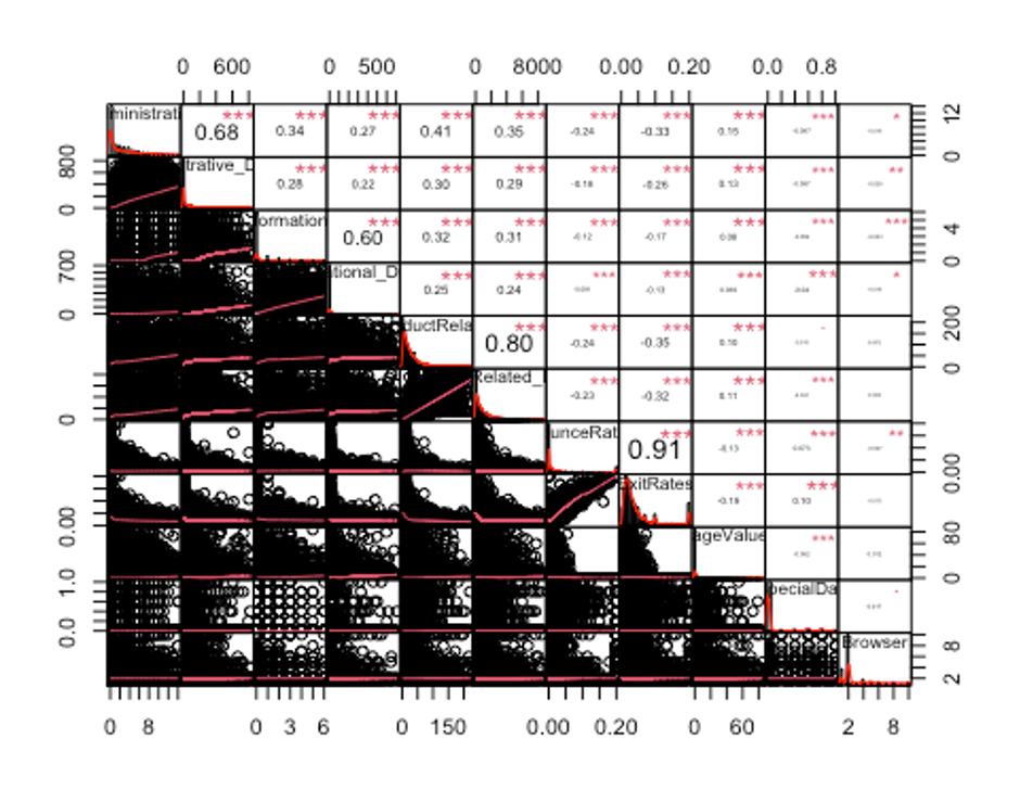
보통 상관계수의 절댓값이 0.7보다 크면 강한 상관관계가 있다고 보고, 0.3보다 크면 약한 상관관계가 있다고 본다. 상관계수가 0.3보다 작으면 일반적으로 상관관계가 없다고 해석한다. 독립변수 간에 선형 상관관계가 존재하는 경우 다중공선성이 있다고 얘기하는데, 다중공선성이 있으면 독립변수 간에 선형상관관계가 있어서 회귀계수의 분산이 커진다. 그 결과 분석 결과가 불안정하게 되어 분석의 효과성이 감소하는 문제가 발생한다.
- 상관관계의 절댓값이 0.7이상인 변수를 제거하자.
findCorrelation(cor_df, cutoff = 0.7)
## [1] 5 8- df_numeric2에서 5번째 변수와 8번째 변수는 각각 ProductRelated변수와 ExitRates변수이므로 이 둘을 df_2에서 제거하자.
df_new <- df_2[, -c(5, 8)]
str(df_new)
## 'data.frame':    12330 obs. of  16 variables:
##  $ Administrative         : num  0 0 0 0 0 0 0 1 0 0 ...
##  $ Administrative_Duration: num  0 0 0 0 0 0 0 0 0 0 ...
##  $ Informational          : num  0 0 0 0 0 0 0 0 0 0 ...
##  $ Informational_Duration : num  0 0 0 0 0 0 0 0 0 0 ...
##  $ ProductRelated_Duration: num  0 64 0 2.67 627.5 ...
##  $ BounceRates            : num  0.2 0 0.2 0.05 0.02 ...
##  $ PageValues             : num  0 0 0 0 0 0 0 0 0 0 ...
##  $ SpecialDay             : num  0 0 0 0 0 0 0.4 0 0.8 0.4 ...
##  $ Browser                : num  1 2 1 2 3 2 4 2 2 4 ...
##  $ Month                  : Factor w/ 10 levels "Feb","Mar","May",..: 1 1 1 1 1 1 1 1 1 1 ...
##  $ OperatingSystems       : Factor w/ 8 levels "1","2","3","4",..: 1 2 4 3 3 2 2 1 2 2 ...
##  $ Region                 : Factor w/ 9 levels "1","2","3","4",..: 1 1 9 2 1 1 3 1 2 1 ...
##  $ TrafficType            : Factor w/ 20 levels "1","2","3","4",..: 1 2 3 4 4 3 3 5 3 2 ...
##  $ VisitorType            : Factor w/ 3 levels "New_Visitor",..: 3 3 3 3 3 3 3 3 3 3 ...
##  $ Weekend                : Factor w/ 2 levels "FALSE","TRUE": 1 1 1 1 2 1 1 2 1 1 ...
## $ Revenue : Factor w/ 2 levels "FALSE","TRUE": 1 1 1 1 1 1 1 1 1 1 ...- 다음으로 분산이 0에 가까운 변수를 제거하자.
nearZeroVar(df_new, saveMetrics = TRUE)
##                           freqRatio percentUnique zeroVar   nzv
## Administrative             4.259970     0.1216545   FALSE FALSE
## Administrative_Duration   47.604839    26.0583942   FALSE FALSE
## Informational              9.396734     0.0567721   FALSE FALSE
## Informational_Duration   304.515152     9.2133009   FALSE  TRUE
## ProductRelated_Duration    6.088710    76.4639092   FALSE FALSE
## BounceRates                7.882857    15.1824818   FALSE FALSE
## PageValues              1620.666667    20.9326845   FALSE FALSE
## SpecialDay                31.564103     0.0486618   FALSE  TRUE
## Browser                    3.264825     0.0811030   FALSE FALSE
## Month                      1.122081     0.0811030   FALSE FALSE
## OperatingSystems           2.553578     0.0648824   FALSE FALSE
## Region                     1.989180     0.0729927   FALSE FALSE
## TrafficType                1.596491     0.1622060   FALSE FALSE
## VisitorType                6.228453     0.0243309   FALSE FALSE
## Weekend                    3.299163     0.0162206   FALSE FALSE
## Revenue                    5.462264     0.0162206   FALSE FALSE
df_new2 <- df_new[, -nearZeroVar(df_new)]
str(df_new2)
## 'data.frame':    12330 obs. of  14 variables:
##  $ Administrative         : num  0 0 0 0 0 0 0 1 0 0 ...
##  $ Administrative_Duration: num  0 0 0 0 0 0 0 0 0 0 ...
##  $ Informational          : num  0 0 0 0 0 0 0 0 0 0 ...
##  $ ProductRelated_Duration: num  0 64 0 2.67 627.5 ...
##  $ BounceRates            : num  0.2 0 0.2 0.05 0.02 ...
##  $ PageValues             : num  0 0 0 0 0 0 0 0 0 0 ...
##  $ Browser                : num  1 2 1 2 3 2 4 2 2 4 ...
##  $ Month                  : Factor w/ 10 levels "Feb","Mar","May",..: 1 1 1 1 1 1 1 1 1 1 ...
##  $ OperatingSystems       : Factor w/ 8 levels "1","2","3","4",..: 1 2 4 3 3 2 2 1 2 2 ...
##  $ Region                 : Factor w/ 9 levels "1","2","3","4",..: 1 1 9 2 1 1 3 1 2 1 ...
##  $ TrafficType            : Factor w/ 20 levels "1","2","3","4",..: 1 2 3 4 4 3 3 5 3 2 ...
##  $ VisitorType            : Factor w/ 3 levels "New_Visitor",..: 3 3 3 3 3 3 3 3 3 3 ...
##  $ Weekend                : Factor w/ 2 levels "FALSE","TRUE": 1 1 1 1 2 1 1 2 1 1 ...
##  $ Revenue                : Factor w/ 2 levels "FALSE","TRUE": 1 1 1 1 1 1 1 1 1 1 ...
Informational_Duration, SpecialDay변수의 분산이 0에 가까운 것으로 나타나 데이터프레임에서 제거하였다.
- 데이터를 train데이터와 test데이터로 분리한다.
idx <- createDataPartition(df_new2$Revenue, p = 0.7)
train <- df[idx$Resample1, ]
test <- df[-idx$Resample1, ]
table(train$Revenue)
##
## FALSE  TRUE
##  7296  1336
결과변수 Revenue의 범주가 약 5.5배 차이로 불균형 데이터이다.
- ROSE(random over sampling examples) 기법을 이용해 불균형 문제를 해결해보자
train_ROSE <- ROSE(Revenue ~., data = train, seed = 123)$data
table(train$Revenue)
##
## FALSE  TRUE
##  7296  1336
table(train_ROSE$Revenue)
##
## FALSE  TRUE
## 4366 4266- 데이터 스케일링을 진행해보자.
model_train <- preProcess(train_ROSE, method = 'range')
model_test <- preProcess(test, method = 'range')
scaled_train_ROSE <- predict(model_train, train_ROSE)
scaled_test <- predict(model_test, test)- factor형 변수들을 더미 변수로 만들어주자.
dummies <- dummyVars(Revenue ~., data = train_ROSE)
train_ROSE_dummy <- as.data.frame(predict(dummies, newdata = train_ROSE))
train_ROSE_dummy$Revenue <- train_ROSE$Revenue

dummies2 <- dummyVars(Revenue ~., data = scaled_train_ROSE)
scaled_train_ROSE_dummy <- as.data.frame(predict(dummies2, newdata = scaled_train_ROSE))
scaled_train_ROSE_dummy$Revenue <- scaled_train_ROSE$Revenue

dummies3 <- dummyVars(Revenue ~., data = test)
test_dummy <- as.data.frame(predict(dummies3, newdata = test))
test_dummy$Revenue <- test$Revenue

dummies4 <- dummyVars(Revenue ~., data = scaled_test)
scaled_test_dummy <- as.data.frame(predict(dummies4, newdata = scaled_test))
scaled_test_dummy$Revenue <- scaled_test$Revenue
세트1 - train_ROSE, test : 데이터스케일X, 더미변수화X
세트2 - scaled_train_ROSE, scaled_test : 데이터스케일O, 더미변수화X
세트3 - train_ROSE_dummy, test_dummy : 데이터스케일X, 더미변수화O
세트4 - scaled_train_ROSE_dummy, scaled_test_dummy : 데이터 스케일O, 더미변수화O
총 4개의 조합이 만들어졌다. 모델 훈련법에 따라 세트를 선택해 사용하자. 다만 모형 훈련에 더미 변수가 들어가면 다른 변수에 비해 과하게 반영될 여지가 있기 때문에 굳이 더미 변수를 사용해야 할 이유가 없다면 사용하지 않는 것이 좋다.
다변량 적응 회귀 스플라인(MARS)
- train_ROSE, test데이터 세트를 사용한다.
- 먼저 필요한 패키지들을 불러오자.
library(MASS)
##
## Attaching package: 'MASS'
## The following object is masked from 'package:dplyr':
##
##     select
library(bestglm)
## Loading required package: leaps
library(earth)
## Loading required package: Formula
## Loading required package: plotmo
## Loading required package: plotrix
##
## Attaching package: 'plotrix'
## The following object is masked from 'package:psych':
##
##     rescale
## Loading required package: TeachingDemos
library(ROCR)
library(car)
## Loading required package: carData
##
## Attaching package: 'car'
## The following object is masked from 'package:dplyr':
##
##     recode
## The following object is masked from 'package:psych':
##
## logit- 모형을 만들어 보자.
set.seed(321)
earth.fit <- earth(Revenue ~., data = train_ROSE,
                   pmethod = 'cv', nfold = 10,
                   ncross = 3, degree = 1,
                   minspan = -1,
                   glm = list(family = binomial))
summary(earth.fit)
## Call: earth(formula=Revenue~., data=train_ROSE, pmethod="cv",
##             glm=list(family=binomial), degree=1, nfold=10, ncross=3,
##             minspan=-1)
##
## GLM coefficients
##                                         TRUE
## (Intercept)                        -0.217794
## MonthMar                           -0.716594
## MonthNov                            0.548364
## MonthDec                           -0.649609
## OperatingSystems2                   0.007544
## TrafficType3                       -0.470470
## TrafficType13                      -0.615791
## VisitorTypeOther                   -1.528098
## VisitorTypeReturning_Visitor       -0.288701
## h(1.82014-Administrative)           0.025182
## h(Administrative-1.82014)           0.026639
## h(53.774-Administrative_Duration)   0.002749
## h(Administrative_Duration-53.774)   0.000967
## h(0.299924-Informational)           0.310813
## h(Informational-0.299924)           0.120581
## h(16.8912-Informational_Duration)   0.005569
## h(Informational_Duration-16.8912)   0.000703
## h(26.4066-ProductRelated)           0.010541
## h(ProductRelated-26.4066)           0.005902
## h(0.00535212-BounceRates)         -95.365506
## h(BounceRates-0.00535212)         -56.603481
## h(0.0220586-ExitRates)            -35.887553
## h(ExitRates-0.0220586)            -34.425075
## h(3.94875-PageValues)               0.097953
## h(PageValues-3.94875)               0.098646
## h(0.00811794-SpecialDay)           -4.593668
## h(SpecialDay-0.00811794)           -1.307738
## h(2.02052-Browser)                  0.347494
## h(Browser-2.02052)                  0.157571
##
## GLM (family binomial, link logit):
##  nulldev   df       dev   df   devratio     AIC iters converged
##  11965.3 8631   5827.97 8603      0.513    5886     7         1
##
## Earth selected 29 of 29 terms, and 18 of 57 predictors (pmethod="cv")
## Termination condition: RSq changed by less than 0.001 at 29 terms
## Importance: PageValues, ExitRates, BounceRates, MonthNov, ...
## Number of terms at each degree of interaction: 1 28 (additive model)
## Earth GRSq 0.3992937  RSq 0.4070635  mean.oof.RSq 0.4035203 (sd 0.017)
##
## pmethod="backward" would have selected:
## 28 terms 18 preds, GRSq 0.3995216 RSq 0.4070119 mean.oof.RSq 0.4015694- plotmo()함수를 이용해 해당 예측 변수를 변화시키고 다른 변수들은 상수로 유지했을 때, 모형의 반응 변수가 변하는 양상을 보자.
plotmo(earth.fit)
##  plotmo grid:    Administrative Administrative_Duration Informational
##                         1.82001                53.75336     0.2998683
##  Informational_Duration ProductRelated ProductRelated_Duration BounceRates
##                16.88521       26.40348                1018.886 0.005349781
##   ExitRates PageValues SpecialDay Month OperatingSystems  Browser Region
##  0.02205257   3.945293 0.00810046   Nov                2 2.020514      1
##  TrafficType       VisitorType Weekend
##            2 Returning_Visitor   FALSE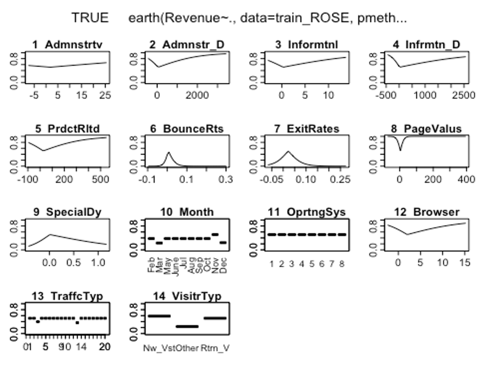
그래프를 보았을 때 OperatingSystems변수의 라벨에 따라서 반응변수가 크게 달라지지 않는 것으로 보인다.
- plotd()함수를 이용해 결과변수 라벨(TRUE/FALSE)에 따른 예측 확률의 밀도 함수 도표를 보자.
plotd(earth.fit)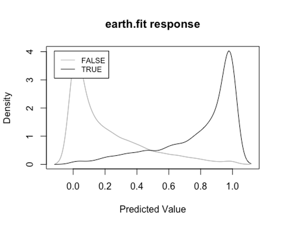
- evimp()함수로 상대적인 변수의 중요도를 살펴보자.
- nsubsets라는 변수명을 볼 수 있는데, 이는 가지치기 패스를 한 후에 남는 변수를 담고 있는 모형의 서브 세트 개수이다.
- gcv와 rss칼럼은 각 예측변수가 기여하는 각 감소값을 나타낸다.
evimp(earth.fit)
##                              nsubsets   gcv    rss
## PageValues                         28 100.0  100.0
## ExitRates                          27  76.3   76.8
## BounceRates                        26  61.8   62.6
## MonthNov                           23  47.0   48.1
## Informational_Duration             22  38.6   40.1
## ProductRelated                     21  37.1   38.6
## SpecialDay                         17  29.3   30.9
## Informational                      16  27.5   29.1
## MonthMar                           15  26.2   27.8
## MonthDec                           15  26.2   27.8
## TrafficType3                       15  26.2   27.8
## TrafficType13                      15  26.2   27.8
## Browser                            11  19.6   21.1
## VisitorTypeOther                    9  17.3   18.8
## VisitorTypeReturning_Visitor        8  15.8   17.3
## Administrative_Duration             7  14.1   15.5
## Administrative                      5  10.6   11.9
## OperatingSystems2                   2   4.5    5.8
PageValues, BounceRates, ExitRates순으로 중요한 변수인 것으로 나타났다.
- test데이터에 모형이 얼마나 잘 작동하는지 보자.
test.earth.fit <- predict(earth.fit, newdata = test, type = 'class')
test.earth.fit <- as.factor(test.earth.fit)
earth.confusion <- confusionMatrix(test.earth.fit, test$Revenue, positive = 'TRUE')
earth.confusion
## Confusion Matrix and Statistics
##
##           Reference
## Prediction FALSE TRUE
##      FALSE  2425  134
##      TRUE    701  438
##
##                Accuracy : 0.7742
##                  95% CI : (0.7604, 0.7876)
##     No Information Rate : 0.8453
##     P-Value [Acc > NIR] : 1
##
##                   Kappa : 0.3854
##
##  Mcnemar's Test P-Value : <2e-16
##
##             Sensitivity : 0.7657
##             Specificity : 0.7758
##          Pos Pred Value : 0.3845
##          Neg Pred Value : 0.9476
##              Prevalence : 0.1547
##          Detection Rate : 0.1184
##    Detection Prevalence : 0.3080
##       Balanced Accuracy : 0.7707
##
##        'Positive' Class : TRUE
##
earth.confusion$byClass
##          Sensitivity          Specificity       Pos Pred Value
##            0.7657343            0.7757518            0.3845478
##       Neg Pred Value            Precision               Recall
##            0.9476358            0.3845478            0.7657343
##                   F1           Prevalence       Detection Rate
##            0.5119813            0.1546782            0.1184424
## Detection Prevalence    Balanced Accuracy
##            0.3080043            0.7707430
MARS모형의 Accuracy는 0.713, Kappa는 0.318, F1-score는 0.468인 것으로 나타났다.
- ROC커브를 그려보자.
test.earth.pred <- predict(earth.fit, newdata = test, type = 'response')
pred.earth <- prediction(test.earth.pred, test$Revenue)
perf.earth <- performance(pred.earth, 'tpr', 'fpr')
plot(perf.earth, col = 1)
legend(0.6, 0.6, c('MARS'), 1)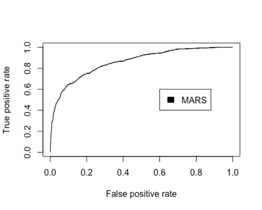
- AUC를 확인해보자.
performance(pred.earth, 'auc')@y.values
## [[1]]
## [1] 0.8597294
MARS모형의 Accuracy는 0.713, Kappa는 0.318, F1-score는 0.468, AUC는 0.860인 것으로 나타났다.
KNN
- K-최근접 이웃법을 이용해 모형을 만들어 보자.
– scaled_train_ROSE_dummy, scaled_test_dummy데이터를 사용한다.
– 먼저 필요한 패키지를 불러오자.
library(class)
library(kknn)
##
## Attaching package: 'kknn'
## The following object is masked from 'package:caret':
##
##     contr.dummy
library(e1071)
##
## Attaching package: 'e1071'
## The following objects are masked from 'package:PerformanceAnalytics':
##
##     kurtosis, skewness
library(kernlab)
##
## Attaching package: 'kernlab'
## The following object is masked from 'package:ggplot2':
##
##     alpha
## The following object is masked from 'package:psych':
##
## alpha- KNN을 사용할 때는 적절한 k를 선택하는 것이 중요하다.
– expand.grid()와 seq()함수를 사용해 k를 선택해보자.
grid1 <- expand.grid(.k = seq(2, 30, by = 1))
control <- trainControl(method = 'cv')
set.seed(321)
knn.train <- train(Revenue ~., data = scaled_train_ROSE_dummy,
                   method = 'knn',
                   trControl = control,
                   tuneGrid = grid1)
knn.train
## k-Nearest Neighbors
##
## 8632 samples
##   63 predictor
##    2 classes: 'FALSE', 'TRUE'
##
## No pre-processing
## Resampling: Cross-Validated (10 fold)
## Summary of sample sizes: 7768, 7769, 7769, 7769, 7768, 7769, ...
## Resampling results across tuning parameters:
##
##   k   Accuracy   Kappa
##    2  0.8111697  0.6227830
##    3  0.8138318  0.6282663
##    4  0.7924007  0.5854331
##    5  0.7857992  0.5723240
##    6  0.7670321  0.5347231
##    7  0.7635546  0.5278156
##    8  0.7526647  0.5060082
##    9  0.7511569  0.5030159
##   10  0.7473340  0.4953649
##   11  0.7453659  0.4914052
##   12  0.7376063  0.4759192
##   13  0.7379528  0.4765999
##   14  0.7322743  0.4652464
##   15  0.7328553  0.4663932
##   16  0.7284531  0.4575663
##   17  0.7276427  0.4558905
##   18  0.7226623  0.4459133
##   19  0.7262530  0.4531177
##   20  0.7254414  0.4514614
##   21  0.7219671  0.4444813
##   22  0.7197677  0.4401064
##   23  0.7190711  0.4386658
##   24  0.7165242  0.4335750
##   25  0.7157120  0.4319530
##   26  0.7157129  0.4319595
##   27  0.7127024  0.4259238
##   28  0.7094565  0.4194906
##   29  0.7106164  0.4217374
##   30  0.7107318  0.4219711
##
## Accuracy was used to select the optimal model using the largest value.
## The final value used for the model was k = 2.
k매개변수 값으로 2가 나왔다.
- knn()함수를 이용해 모형을 만들어 보자.
knn.model <- knn(scaled_train_ROSE_dummy[, -64], scaled_test_dummy[, -64], scaled_train_ROSE_dummy[, 64], k = 2)
summary(knn.model)
## FALSE  TRUE
## 2539 1159- scaled_test_dummy를 이용해 모형이 잘 작동하는지 보자.
knn.confusion <- confusionMatrix(knn.model, scaled_test_dummy$Revenue, positive = 'TRUE')
knn.confusion
## Confusion Matrix and Statistics
##
##           Reference
## Prediction FALSE TRUE
##      FALSE  2230  309
##      TRUE    896  263
##
##                Accuracy : 0.6741
##                  95% CI : (0.6588, 0.6892)
##     No Information Rate : 0.8453
##     P-Value [Acc > NIR] : 1
##
##                   Kappa : 0.122
##
##  Mcnemar's Test P-Value : <2e-16
##
##             Sensitivity : 0.45979
##             Specificity : 0.71337
##          Pos Pred Value : 0.22692
##          Neg Pred Value : 0.87830
##              Prevalence : 0.15468
##          Detection Rate : 0.07112
##    Detection Prevalence : 0.31341
##       Balanced Accuracy : 0.58658
##
##        'Positive' Class : TRUE
##
knn.confusion$byClass
##          Sensitivity          Specificity       Pos Pred Value
##           0.45979021           0.71337172           0.22691976
##       Neg Pred Value            Precision               Recall
##           0.87829854           0.22691976           0.45979021
##                   F1           Prevalence       Detection Rate
##           0.30387060           0.15467820           0.07111952
## Detection Prevalence    Balanced Accuracy
##           0.31341266           0.58658097
Accuracy : 0.678, Kappa : 0.113, F1-score : 0.294의 성능이 나왔다.
- 성능을 올리기 위해 커널을 입력하자.
– distance = 2를 이용해 절댓값합 거리를 사용하자.
kknn.train <- train.kknn(Revenue ~., data = scaled_train_ROSE_dummy, kmax = 30, distance = 2,
                         kernel = c('rectangular', 'triangular', 'epanechnikov', 'cosine', 'gaussian', 'optimal'))
plot(kknn.train)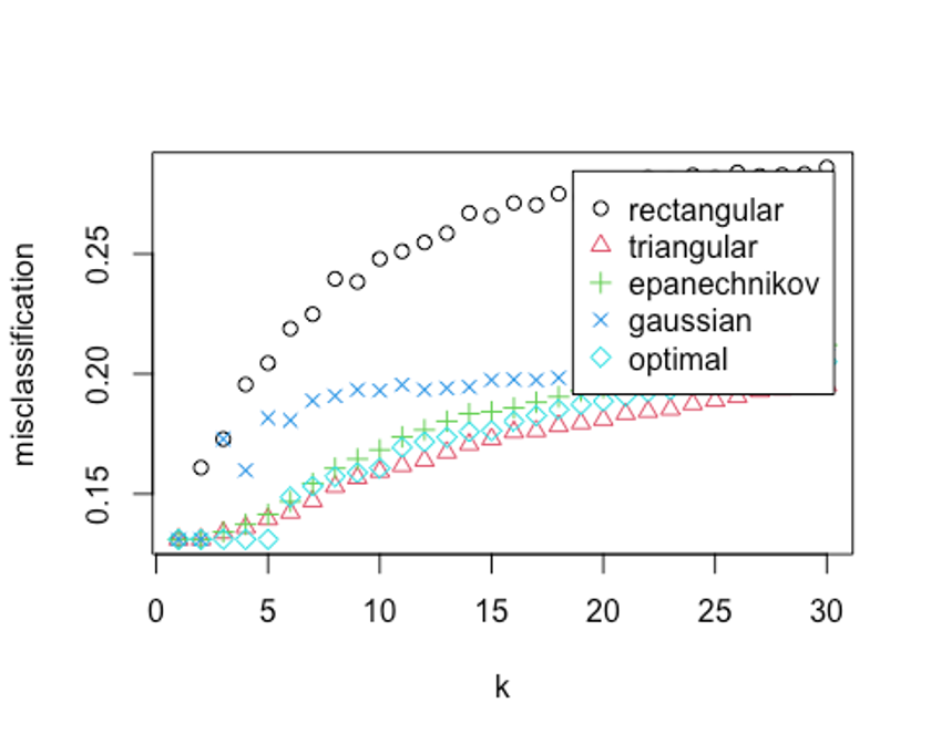
- 자세한 값을 살펴보자.
kknn.train
##
## Call:
## train.kknn(formula = Revenue ~ ., data = scaled_train_ROSE_dummy,     kmax = 30, distance = 2, kernel = c("rectangular", "triangular",         "epanechnikov", "cosine", "gaussian", "optimal"))
##
## Type of response variable: nominal
## Minimal misclassification: 0.1310241
## Best kernel: rectangular
## Best k: 1
k = 1, rectangular커널을 사용했을 때 약 13%의 오류가 나온 것으로 나타났다.
- distance = 1을 사용해 유클리드 거리로 다시 측정해보자.
kknn.train2 <- train.kknn(Revenue ~., data = scaled_train_ROSE_dummy, kmax = 30, distance = 1,
                         kernel = c('rectangular', 'triangular', 'epanechnikov', 'cosine', 'gaussian', 'optimal'))
plot(kknn.train2)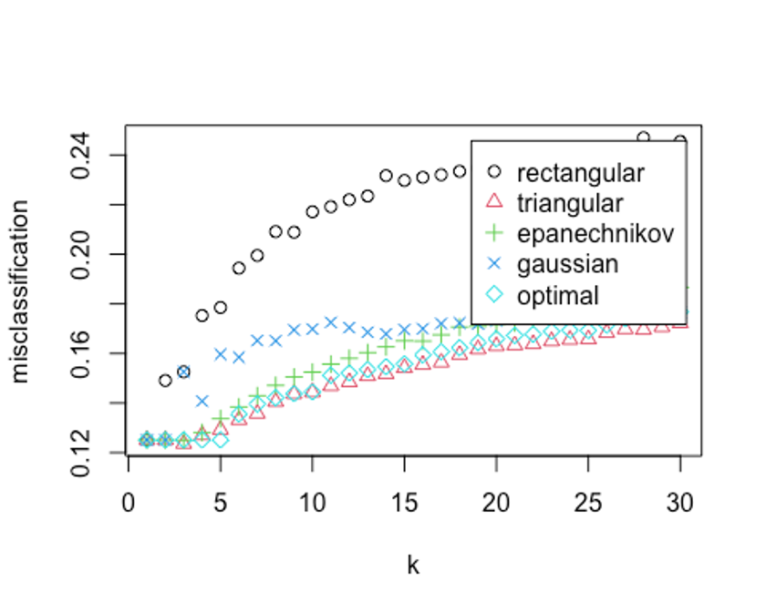
kknn.train2
##
## Call:
## train.kknn(formula = Revenue ~ ., data = scaled_train_ROSE_dummy,     kmax = 30, distance = 1, kernel = c("rectangular", "triangular",         "epanechnikov", "cosine", "gaussian", "optimal"))
##
## Type of response variable: nominal
## Minimal misclassification: 0.1236098
## Best kernel: triangular
## Best k: 3
오류율이 더 떨어졌다. 최종 knn 하이퍼 파라미터로 유클리드 거리를 사용하고, k가 3, triangular커널을 사용하자.
- 예측 성능을 보자.
kknn.fit <- predict(kknn.train2, newdata = scaled_test_dummy)
kknn.fit <- as.factor(kknn.fit)
kknn.confusion <- confusionMatrix(kknn.fit, scaled_test_dummy$Revenue, positive = 'TRUE')
kknn.confusion
## Confusion Matrix and Statistics
##
##           Reference
## Prediction FALSE TRUE
##      FALSE  2315  314
##      TRUE    811  258
##
##                Accuracy : 0.6958
##                  95% CI : (0.6807, 0.7106)
##     No Information Rate : 0.8453
##     P-Value [Acc > NIR] : 1
##
##                   Kappa : 0.1414
##
##  Mcnemar's Test P-Value : <2e-16
##
##             Sensitivity : 0.45105
##             Specificity : 0.74056
##          Pos Pred Value : 0.24135
##          Neg Pred Value : 0.88056
##              Prevalence : 0.15468
##          Detection Rate : 0.06977
##    Detection Prevalence : 0.28908
##       Balanced Accuracy : 0.59581
##
##        'Positive' Class : TRUE
##
kknn.confusion$byClass
##          Sensitivity          Specificity       Pos Pred Value
##           0.45104895           0.74056302           0.24134705
##       Neg Pred Value            Precision               Recall
##           0.88056295           0.24134705           0.45104895
##                   F1           Prevalence       Detection Rate
##           0.31444241           0.15467820           0.06976744
## Detection Prevalence    Balanced Accuracy
##           0.28907518           0.59580599
Accuracy : 0.690, Kappa : 0.121, F1-score : 0.298의 성능이 나왔다.
- ROC커브를 그려보자.
plot(perf.earth, col = 1)

knn.pred <- predict(kknn.train2, newdata = scaled_test_dummy, type = 'prob')
head(knn.pred)
##      FALSE TRUE
## [1,]     1    0
## [2,]     1    0
## [3,]     1    0
## [4,]     1    0
## [5,]     1    0
## [6,]     1    0
knn.pred.true <- knn.pred[, 2]
pred.knn <- prediction(knn.pred.true, scaled_test_dummy$Revenue)
perf.knn <- performance(pred.knn, 'tpr', 'fpr')

plot(perf.knn, col = 2, add = TRUE)
legend(0.6, 0.6, c('MARS', 'KNN'), 1:2)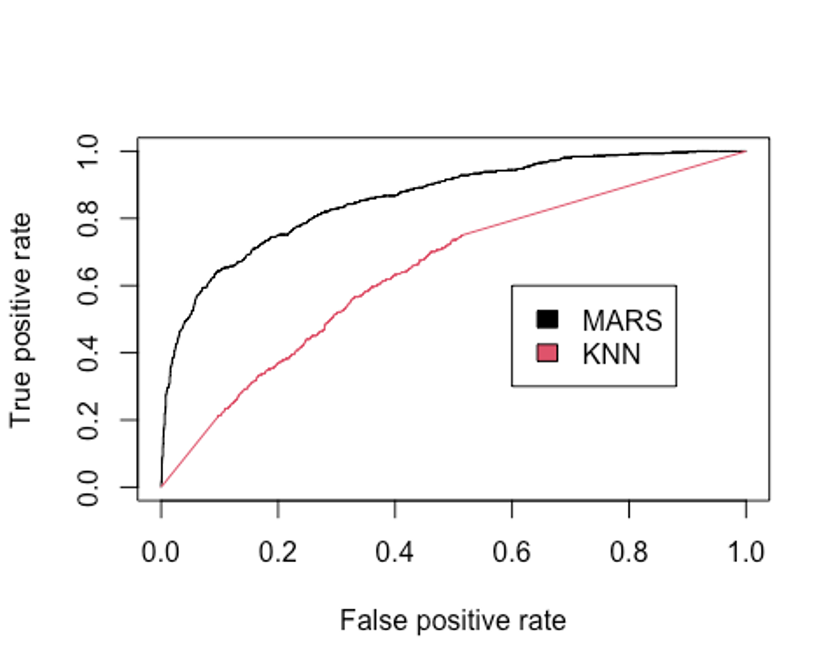
- AUC를 알아보자.
performance(pred.earth, 'auc')@y.values
## [[1]]
## [1] 0.8597294
performance(pred.knn, 'auc')@y.values
## [[1]]
## [1] 0.6454863
KNN모형이 MARS모형보다 현저히 성능이 떨어지는 것으로 나타났다.
SVM
- 다음으로 SVM모형을 만들어 보자.
– scaled_train_ROSE, scaled_test를 사용한다.
– 선형 SVM모형부터 만들어보자.
– tune.svm()함수를 사용해 파라미터를 튜닝하고 커널 함수를 선택해 보자.
set.seed(321)
linear.tune <- tune.svm(Revenue ~., data = scaled_train_ROSE, kernel = 'linear',
                        cost = c(0.001, 0.01, 0.05, 0.1, 0.5, 1, 2, 5, 10))
summary(linear.tune)
##
## Parameter tuning of 'svm':
##
## - sampling method: 10-fold cross validation
##
## - best parameters:
##  cost
##   0.5
##
## - best performance: 0.2438627
##
## - Detailed performance results:
##    cost     error dispersion
## 1 1e-03 0.2546346 0.01065937
## 2 1e-02 0.2445572 0.01319503
## 3 5e-02 0.2447894 0.01512409
## 4 1e-01 0.2445572 0.01444559
## 5 5e-01 0.2438627 0.01488985
## 6 1e+00 0.2442100 0.01432033
## 7 2e+00 0.2442101 0.01424995
## 8 5e+00 0.2445578 0.01443419
## 9 1e+01 0.2447893 0.01423905
이 문제에서 최적의 cost함수는 0.5로 나왔고, 분류 오류 비율은 대략 24.3%이다.
- predict()함수로 scaled_test데이터 예측을 실행해보자.
best.linear <- linear.tune$best.model
tune.fit <- predict(best.linear, newdata = scaled_test, type = 'class')
tune.fit <- as.factor(tune.fit)
linear.svm.confusion <- confusionMatrix(tune.fit, scaled_test$Revenue, positive = 'TRUE')
linear.svm.confusion
## Confusion Matrix and Statistics
##
##           Reference
## Prediction FALSE TRUE
##      FALSE  3110  465
##      TRUE     16  107
##
##                Accuracy : 0.8699
##                  95% CI : (0.8587, 0.8806)
##     No Information Rate : 0.8453
##     P-Value [Acc > NIR] : 1.301e-05
##
##                   Kappa : 0.2678
##
##  Mcnemar's Test P-Value : < 2.2e-16
##
##             Sensitivity : 0.18706
##             Specificity : 0.99488
##          Pos Pred Value : 0.86992
##          Neg Pred Value : 0.86993
##              Prevalence : 0.15468
##          Detection Rate : 0.02893
##    Detection Prevalence : 0.03326
##       Balanced Accuracy : 0.59097
##
##        'Positive' Class : TRUE
##
linear.svm.confusion$byClass
##          Sensitivity          Specificity       Pos Pred Value
##           0.18706294           0.99488164           0.86991870
##       Neg Pred Value            Precision               Recall
##           0.86993007           0.86991870           0.18706294
##                   F1           Prevalence       Detection Rate
##           0.30791367           0.15467820           0.02893456
## Detection Prevalence    Balanced Accuracy
##           0.03326122           0.59097229
Accuracy : 0.870, Kappa : 0.268, F1-score : 0.308의 성능이 나왔다.
- 비선형 방법을 이용해 성능을 더 높혀보자.
– 먼저 polynomial커널함수를 적용해보자.
– polynomial의 차수는 2, 3, 4, 5의 값을 주고, 커널 계수는 0.1부터 4의 값을 준다.
set.seed(321)
poly.tune <- tune.svm(Revenue ~., data = scaled_train_ROSE,
                      kernel = 'polynomial',
                      degree = c(2, 3, 4, 5),
                      coef0 = c(0.1, 0.5, 1, 2, 3, 4))
summary(poly.tune)
##
## Parameter tuning of 'svm':
##
## - sampling method: 10-fold cross validation
##
## - best parameters:
##  degree coef0
##       5     3
##
## - best performance: 0.1244228
##
## - Detailed performance results:
##    degree coef0     error  dispersion
## 1       2   0.1 0.2136248 0.011477565
## 2       3   0.1 0.2238190 0.009216139
## 3       4   0.1 0.2569478 0.017482042
## 4       5   0.1 0.3772197 0.067941242
## 5       2   0.5 0.2151309 0.009976831
## 6       3   0.5 0.2025036 0.012627937
## 7       4   0.5 0.1974070 0.015111708
## 8       5   0.5 0.1961331 0.014705826
## 9       2   1.0 0.2167530 0.010793538
## 10      3   1.0 0.1921929 0.014408994
## 11      4   1.0 0.1719198 0.013520288
## 12      5   1.0 0.1539638 0.011488268
## 13      2   2.0 0.2183747 0.011273876
## 14      3   2.0 0.1784065 0.014240946
## 15      4   2.0 0.1452737 0.011683276
## 16      5   2.0 0.1292888 0.015147768
## 17      2   3.0 0.2176798 0.011264743
## 18      3   3.0 0.1726146 0.012825017
## 19      4   3.0 0.1384393 0.013437336
## 20      5   3.0 0.1244228 0.012136994
## 21      2   4.0 0.2176799 0.011201394
## 22      3   4.0 0.1672857 0.014499167
## 23      4   4.0 0.1363551 0.015486386
## 24      5   4.0 0.1275511 0.011526925
이 모형은 다항식의 차수 degree의 값으로 5, 커널계수는 3을 선택했다.
- scaled_test데이터로 예측을 해보자.
best.poly <- poly.tune$best.model
poly.test <- predict(best.poly, newdata = scaled_test, type = 'class')
poly.test <- as.factor(poly.test)
poly.svm.confusion <- confusionMatrix(poly.test, scaled_test$Revenue, positive = 'TRUE')
poly.svm.confusion
## Confusion Matrix and Statistics
##
##           Reference
## Prediction FALSE TRUE
##      FALSE  1161  290
##      TRUE   1965  282
##
##                Accuracy : 0.3902
##                  95% CI : (0.3744, 0.4061)
##     No Information Rate : 0.8453
##     P-Value [Acc > NIR] : 1
##
##                   Kappa : -0.0617
##
##  Mcnemar's Test P-Value : <2e-16
##
##             Sensitivity : 0.49301
##             Specificity : 0.37140
##          Pos Pred Value : 0.12550
##          Neg Pred Value : 0.80014
##              Prevalence : 0.15468
##          Detection Rate : 0.07626
##    Detection Prevalence : 0.60763
##       Balanced Accuracy : 0.43220
##
##        'Positive' Class : TRUE
##
poly.svm.confusion$byClass
##          Sensitivity          Specificity       Pos Pred Value
##           0.49300699           0.37140115           0.12550067
##       Neg Pred Value            Precision               Recall
##           0.80013784           0.12550067           0.49300699
##                   F1           Prevalence       Detection Rate
##           0.20007095           0.15467820           0.07625744
## Detection Prevalence    Balanced Accuracy
##           0.60762574           0.43220407
Accuracy : 0.390, Kappa : -0.062, F1-score : 0.200의 성능이 나왔다. 선형 SVM모델보다 성능이 떨어진다.
- 다음으로 방사 기저 함수를 커널로 설정해보자.
– 매개변수는 gamma로 최적값을 찾기위해 0.01부터 4까지 증가시켜 본다.
– gamma값이 너무 작을 때는 모형이 결정분계선을 제대로 포착하지 못할 수도 있고, 값이 너무 클 때는 모형이 지나치게 과적합될 수 있으므로 주의가 필요하다.
set.seed(321)
rbf.tune <- tune.svm(Revenue ~., data = scaled_train_ROSE,
                     kernel = 'radial',
                     gamma = c(0.01, 0.05, 0.1, 0.5, 1, 2, 3, 4))
summary(rbf.tune)
##
## Parameter tuning of 'svm':
##
## - sampling method: 10-fold cross validation
##
## - best parameters:
##  gamma
##    0.1
##
## - best performance: 0.133227
##
## - Detailed performance results:
##   gamma     error dispersion
## 1  0.01 0.2209232 0.01139738
## 2  0.05 0.1594092 0.01383613
## 3  0.10 0.1332270 0.01325140
## 4  0.50 0.1342693 0.01149102
## 5  1.00 0.1789874 0.01099134
## 6  2.00 0.4136877 0.02304142
## 7  3.00 0.4829677 0.01365227
## 8  4.00 0.4904989 0.01121232
최적의 gamma값은 0.1이다.
- 마찬가지로 성능을 예측해보자.
best.rbf <- rbf.tune$best.model
rbf.test <- predict(best.rbf, newdata = scaled_test, type = 'class')
rbf.test <- as.factor(rbf.test)
rbf.svm.confusion <- confusionMatrix(rbf.test, scaled_test$Revenue, positive = 'TRUE')
rbf.svm.confusion
## Confusion Matrix and Statistics
##
##           Reference
## Prediction FALSE TRUE
##      FALSE   122   57
##      TRUE   3004  515
##
##                Accuracy : 0.1723
##                  95% CI : (0.1602, 0.1848)
##     No Information Rate : 0.8453
##     P-Value [Acc > NIR] : 1
##
##                   Kappa : -0.0195
##
##  Mcnemar's Test P-Value : <2e-16
##
##             Sensitivity : 0.90035
##             Specificity : 0.03903
##          Pos Pred Value : 0.14635
##          Neg Pred Value : 0.68156
##              Prevalence : 0.15468
##          Detection Rate : 0.13926
##    Detection Prevalence : 0.95160
##       Balanced Accuracy : 0.46969
##
##        'Positive' Class : TRUE
##
rbf.svm.confusion$byClass
##          Sensitivity          Specificity       Pos Pred Value
##           0.90034965           0.03902751           0.14634839
##       Neg Pred Value            Precision               Recall
##           0.68156425           0.14634839           0.90034965
##                   F1           Prevalence       Detection Rate
##           0.25177218           0.15467820           0.13926447
## Detection Prevalence    Balanced Accuracy
##           0.95159546           0.46968858
Accuracy : 0.172, Kappa : -0.195, F1-score : 0.252의 성능이 나왔다.
- 다시 성능 개선을 위해 sigmoid함수로 설정해보자.
– 매개변수인 gamma와 coef0이 최적의 값이 되도록 계산해보자.
set.seed(321)
sigmoid.tune <- tune.svm(Revenue ~., data = scaled_train_ROSE,
                         kernel = 'sigmoid',
                         gamma = c(0.1, 0.5, 1, 2, 3, 4),
                         coef0 = c(0.1, 0.5, 1, 2, 3, 4))
summary(sigmoid.tune)
##
## Parameter tuning of 'svm':
##
## - sampling method: 10-fold cross validation
##
## - best parameters:
##  gamma coef0
##    0.1     4
##
## - best performance: 0.3468407
##
## - Detailed performance results:
##    gamma coef0     error dispersion
## 1    0.1   0.1 0.3723386 0.01751505
## 2    0.5   0.1 0.4221501 0.01779125
## 3    1.0   0.1 0.4336186 0.01507837
## 4    2.0   0.1 0.4623463 0.03823503
## 5    3.0   0.1 0.4577106 0.03611425
## 6    4.0   0.1 0.4521562 0.02767209
## 7    0.1   0.5 0.4016492 0.02395204
## 8    0.5   0.5 0.4490297 0.01701384
## 9    1.0   0.5 0.4471733 0.01441787
## 10   2.0   0.5 0.4771777 0.04066548
## 11   3.0   0.5 0.4478606 0.02883916
## 12   4.0   0.5 0.4662848 0.03207388
## 13   0.1   1.0 0.4244720 0.02387098
## 14   0.5   1.0 0.4713884 0.02291624
## 15   1.0   1.0 0.4677966 0.01943992
## 16   2.0   1.0 0.4695354 0.03100309
## 17   3.0   1.0 0.4889955 0.04213662
## 18   4.0   1.0 0.4745028 0.04511312
## 19   0.1   2.0 0.4472937 0.01638526
## 20   0.5   2.0 0.4969898 0.02164017
## 21   1.0   2.0 0.4832031 0.02169763
## 22   2.0   2.0 0.4711563 0.01952145
## 23   3.0   2.0 0.4698815 0.02713059
## 24   4.0   2.0 0.5048693 0.02830511
## 25   0.1   3.0 0.4187918 0.01903577
## 26   0.5   3.0 0.5186545 0.02377845
## 27   1.0   3.0 0.5048649 0.01550109
## 28   2.0   3.0 0.4777603 0.02428690
## 29   3.0   3.0 0.4717361 0.01963229
## 30   4.0   3.0 0.5007038 0.02914465
## 31   0.1   4.0 0.3468407 0.03217296
## 32   0.5   4.0 0.5217822 0.01849434
## 33   1.0   4.0 0.5142523 0.02199626
## 34   2.0   4.0 0.4870263 0.02597384
## 35   3.0   4.0 0.4747484 0.02173184
## 36   4.0   4.0 0.4811119 0.03115664
최적의 gamma값은 0.1이고, coef0값은 4이다.
- 예측을 해보자.
best.sigmoid <- sigmoid.tune$best.model
sigmoid.test <- predict(best.sigmoid, newdata = scaled_test, type = 'class')
sigmoid.test <- as.factor(sigmoid.test)
sigmoid.svm.confusion <- confusionMatrix(sigmoid.test, scaled_test$Revenue, positive = 'TRUE')
sigmoid.svm.confusion
## Confusion Matrix and Statistics
##
##           Reference
## Prediction FALSE TRUE
##      FALSE  3069  511
##      TRUE     57   61
##
##                Accuracy : 0.8464
##                  95% CI : (0.8344, 0.8579)
##     No Information Rate : 0.8453
##     P-Value [Acc > NIR] : 0.4388
##
##                   Kappa : 0.1308
##
##  Mcnemar's Test P-Value : <2e-16
##
##             Sensitivity : 0.10664
##             Specificity : 0.98177
##          Pos Pred Value : 0.51695
##          Neg Pred Value : 0.85726
##              Prevalence : 0.15468
##          Detection Rate : 0.01650
##    Detection Prevalence : 0.03191
##       Balanced Accuracy : 0.54420
##
##        'Positive' Class : TRUE
##
sigmoid.svm.confusion$byClass
##          Sensitivity          Specificity       Pos Pred Value
##           0.10664336           0.98176583           0.51694915
##       Neg Pred Value            Precision               Recall
##           0.85726257           0.51694915           0.10664336
##                   F1           Prevalence       Detection Rate
##           0.17681159           0.15467820           0.01649540
## Detection Prevalence    Balanced Accuracy
##           0.03190914           0.54420460
Accuracy : 0.846, Kappa : 0.131, F1-score : 0.177의 성능이 나왔다.
- 가장 좋은 성능을 보인 sigmoid 함수를 사용한 SVM의 ROC그래프를 그려보자.
set.seed(321)
sigmoid.model <- svm(Revenue ~., data = scaled_train_ROSE, kernel = 'sigmoid', gamma = 0.1, coef0 = 0.1, scale = FALSE, probability = TRUE)

pred_svm <- predict(sigmoid.model, scaled_test, probability = TRUE)
prob <- attr(pred_svm, 'probabilities')
head(prob)
##        FALSE       TRUE
## 4  0.9718696 0.02813039
## 5  0.8936604 0.10633958
## 9  0.9026196 0.09738039
## 10 0.7246909 0.27530908
## 13 0.8644836 0.13551642
## 17 0.9846849 0.01531511
pred.svm <- prediction(prob[, 2], scaled_test$Revenue)
perf.svm <- performance(pred.svm, 'tpr', 'fpr')

plot(perf.earth, col = 1)
plot(perf.knn, col = 2, add = TRUE)
plot(perf.svm, col = 3, add = TRUE)
legend(0.6, 0.6, c('MARS', 'KNN', 'SVM'), 1:3)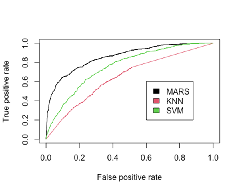
- AUC를 알아보자.
performance(pred.earth, 'auc')@y.values
## [[1]]
## [1] 0.8597294
performance(pred.knn, 'auc')@y.values
## [[1]]
## [1] 0.6454863
performance(pred.svm, 'auc')@y.values
## [[1]]
## [1] 0.7590371
AUC를 보면 MARS, SVM, KNN모형 순으로 성능이 좋다.
Random Forest
- 랜덤포레스트 모델을 만들자.
– train, test데이터를 사용해보자.
– 필요한 패키지를 불러오자.
library(rpart)
library(partykit)
## Loading required package: grid
## Loading required package: libcoin
## Loading required package: mvtnorm
library(genridge)
##
## Attaching package: 'genridge'
## The following object is masked from 'package:bestglm':
##
##     Detroit
## The following object is masked from 'package:caret':
##
##     precision
library(randomForest)
## randomForest 4.7-1
## Type rfNews() to see new features/changes/bug fixes.
##
## Attaching package: 'randomForest'
## The following object is masked from 'package:dplyr':
##
##     combine
## The following object is masked from 'package:gridExtra':
##
##     combine
## The following object is masked from 'package:ggplot2':
##
##     margin
## The following object is masked from 'package:psych':
##
##     outlier
library(xgboost)
##
## Attaching package: 'xgboost'
## The following object is masked from 'package:dplyr':
##
## slice- 기본 모형을 만들어 보자.
set.seed(321)
rf.model <- randomForest(Revenue ~., data = train)
rf.model
##
## Call:
##  randomForest(formula = Revenue ~ ., data = train)
##                Type of random forest: classification
##                      Number of trees: 500
## No. of variables tried at each split: 4
##
##         OOB estimate of  error rate: 9.68%
## Confusion matrix:
##       FALSE TRUE class.error
## FALSE  6999  297  0.04070724
## TRUE    565  771  0.42290419
수행 결과 OOB오차율이 9.68%로 나왔다.
- 개선을 위해 최적의 트리 수를 보자.
plot(rf.model)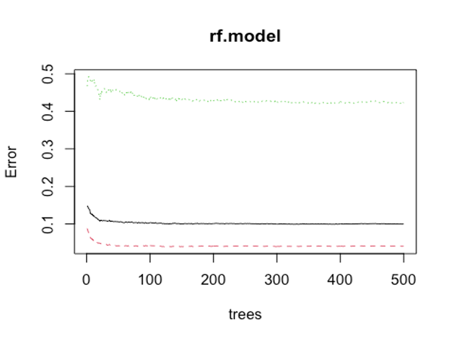
which.min(rf.model$err.rate[, 1])
## [1] 320
모형 정확도를 최적화 하기에 필요한 트리 수가 320개면 된다는 결과를 얻었다.
- 다시 모형을 만들어 보자.
set.seed(321)
rf.model2 <- randomForest(Revenue ~., data = train, ntree = 320)
rf.model2
##
## Call:
##  randomForest(formula = Revenue ~ ., data = train, ntree = 320)
##                Type of random forest: classification
##                      Number of trees: 320
## No. of variables tried at each split: 4
##
##         OOB estimate of  error rate: 9.59%
## Confusion matrix:
##       FALSE TRUE class.error
## FALSE  7001  295  0.04043311
## TRUE    567  769  0.42440120
OOB오차율이 9.68%에서 9.59%로 약간 떨어졌다.
- test데이터로 어떤 결과가 나오는지 보자.
rf.fit <- predict(rf.model2, newdata = test, type = 'class')
rf.fit <- as.factor(rf.fit)
rf.confusion <- confusionMatrix(rf.fit, test$Revenue, positive = 'TRUE')
rf.confusion
## Confusion Matrix and Statistics
##
##           Reference
## Prediction FALSE TRUE
##      FALSE  3012  222
##      TRUE    114  350
##
##                Accuracy : 0.907
##                  95% CI : (0.8994, 0.9182)
##     No Information Rate : 0.8453
##     P-Value [Acc > NIR] : < 2.2e-16
##
##                   Kappa : 0.6179
##
##  Mcnemar's Test P-Value : 5.304e-09
##
##             Sensitivity : 0.61189
##             Specificity : 0.96353
##          Pos Pred Value : 0.75431
##          Neg Pred Value : 0.93135
##              Prevalence : 0.15468
##          Detection Rate : 0.09465
##    Detection Prevalence : 0.12547
##       Balanced Accuracy : 0.78771
##
##        'Positive' Class : TRUE
##
rf.confusion$byClass
##          Sensitivity          Specificity       Pos Pred Value
##           0.61188811           0.96353167           0.75431034
##       Neg Pred Value            Precision               Recall
##           0.93135436           0.75431034           0.61188811
##                   F1           Prevalence       Detection Rate
##           0.67207568           0.15467820           0.09464575
## Detection Prevalence    Balanced Accuracy
##           0.12547323           0.78770989
Accuracy : 0.907, Kappa : 0.618, F1-score : 0.672의 성능이 나왔다.
하이퍼 파마미터 조정 없이도 지금까지 만든 모형 중 최고의 성능을 보이고 있다.
- 성능을 좀 더 높여보자.
rf_mtry <- seq(4, ncol(train)*0.8, by = 2)
rf_nodesize <- seq(3, 8, by = 1)
rf_sample_size <- nrow(train) * c(0.7, 0.8)
rf_hyper_grid <- expand.grid(mtry = rf_mtry,
                             nodesize = rf_nodesize,
samplesize = rf_sample_size)- 설정된 파라미터를 바탕으로 모형을 적합한다.
rf_oob_err <- c()
for(i in 1:nrow(rf_hyper_grid)) {

  model <- randomForest(Revenue ~., data = train,
                        mtry = rf_hyper_grid$mtry[i],
                        nodesize = rf_hyper_grid$nodesize[i],
                        samplesize = rf_hyper_grid$samplesize[i])

  rf_oob_err[i] <- model$err.rate[nrow(model$err.rate), 'OOB']
}- 최적의 하이퍼 파라미터를 보자.
rf_hyper_grid[which.min(rf_oob_err), ]
##    mtry nodesize samplesize
## 55 4 7 6905.6- 위의 파라미터를 토대로 모형을 만들자.
rf_best_model <- randomForest(Revenue ~., data = train,
                              mtry = 4,
                              nodesize = 7,
                              samplesize = 6905.6,
                              proximity = TRUE,
importance = TRUE)- predict()함수로 예측을 해보자.
rf.predict <- predict(rf_best_model, newdata = test, type = 'class')
rf.predict <- as.factor(rf.predict)
rf.best.confusion <- confusionMatrix(rf.predict, test$Revenue, positive = 'TRUE')
rf.best.confusion
## Confusion Matrix and Statistics
##
##           Reference
## Prediction FALSE TRUE
##      FALSE  3020  226
##      TRUE    106  346
##
##                Accuracy : 0.9102
##                  95% CI : (0.9005, 0.9192)
##     No Information Rate : 0.8453
##     P-Value [Acc > NIR] : < 2.2e-16
##
##                   Kappa : 0.6245
##
##  Mcnemar's Test P-Value : 6.534e-11
##
##             Sensitivity : 0.60490
##             Specificity : 0.96609
##          Pos Pred Value : 0.76549
##          Neg Pred Value : 0.93038
##              Prevalence : 0.15468
##          Detection Rate : 0.09356
##    Detection Prevalence : 0.12223
##       Balanced Accuracy : 0.78549
##
##        'Positive' Class : TRUE
##
rf.best.confusion$byClass
##          Sensitivity          Specificity       Pos Pred Value
##           0.60489510           0.96609085           0.76548673
##       Neg Pred Value            Precision               Recall
##           0.93037585           0.76548673           0.60489510
##                   F1           Prevalence       Detection Rate
##           0.67578125           0.15467820           0.09356409
## Detection Prevalence    Balanced Accuracy
##           0.12222823           0.78549298
Accuracy : 0.910, Kappa : 0.625, F1-score : 0.676의 성능이 나왔다. F1-score를 성능 평가의 기준으로 본다면 기본 랜덤 포레스트 모델보다 성능이 약간 더 올라갔다.
- 변수 중요도를 보자.
varImpPlot(rf_best_model, type = 1)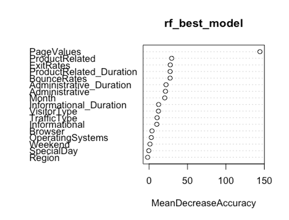
PageValues, ExitRates, ProductRelated, BounceRates순으로 중요한 변수인 것으로 나타났다.
- type를 바꿔서 변수 중요도를 보자.
varImpPlot(rf_best_model, type = 2)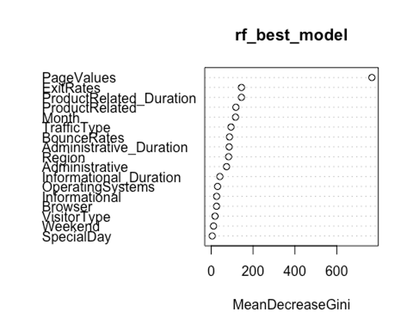
여기서는 PageValues, ExitRates, ProductRelated_Duration, Month순으로 중요한 변수인 것으로 나타났다.
첫번째 plot을 보자. 변수의 값을 랜덤하게 섞었다면, 모델의 정확도가 감소하는 정도를 측정한다.(type = 1)
변수를 랜덤하게 섞는다는 것은 해당 변수가 예측에 미치는 모든 영향력을 제거하는 것을 의미한다. 정확도는 OOB데이터로부터 얻는다. 이는 결국 교차 타당성과 같은 효과를 얻는다.
두번째 plot을 보자. 특정 변수를 기준으로 분할이 일어난 모든 노드에서 불순도 점수의 평균 감소량을 측정한다.(type = 2)
이 지표는 해당 변수가 노드의 불순도를 개선하는데 얼마나 기여했는지를 나타낸다.
그러나 이 지표는 학습데이터를 기반으로 측정되기 때문에 OOB데이터를 가지고 계산한 것에 비해 믿을 만하지 않다.
우리의 plot에서 첫번째와 두번째 plot의 변수 중요도 순서가 다소 다른 것을 볼 수 있는데, OOB데이터로부터 정확도 감소량을 측정한 첫번째 plot이 더 믿을 만하다.
- 랜덤포레스트 모형의 ROC그래프를 그려보자.
rf.pred <- predict(rf_best_model, newdata = test, type = 'prob')
head(rf.pred)
##    FALSE  TRUE
## 4  0.998 0.002
## 5  1.000 0.000
## 9  1.000 0.000
## 10 0.980 0.020
## 13 1.000 0.000
## 17 1.000 0.000
rf.pred.true <- rf.pred[, 2]
pred.rf <- prediction(rf.pred.true, test$Revenue)
perf.rf <- performance(pred.rf, 'tpr', 'fpr')

plot(perf.earth, col = 1)
plot(perf.knn, col = 2, add = TRUE)
plot(perf.svm, col = 3, add = TRUE)
plot(perf.rf, col = 4, add = TRUE)
legend(0.6, 0.6, c('MARS', 'KNN', 'SVM', 'RF'), 1:4)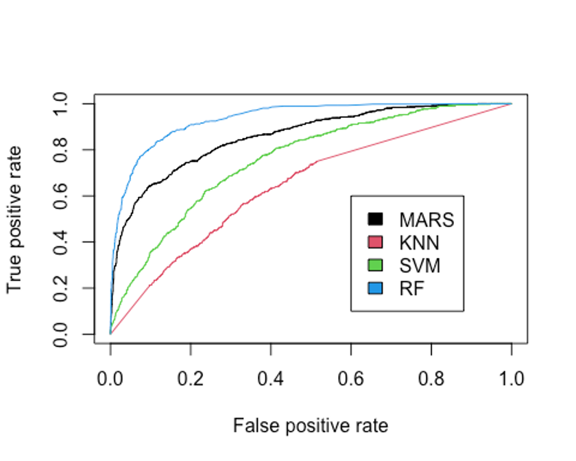
- AUC를 보자.
performance(pred.earth, 'auc')@y.values
## [[1]]
## [1] 0.8597294
performance(pred.knn, 'auc')@y.values
## [[1]]
## [1] 0.6454863
performance(pred.svm, 'auc')@y.values
## [[1]]
## [1] 0.7590371
performance(pred.rf, 'auc')@y.values
## [[1]]
## [1] 0.9365532
랜덤포레스트 모형의 AUC는 0.937, F1-score는 0.676으로 지금까지 만든 모형 중 가장 좋은 성능을 보인다.
XGBoost
- XGBoost모형을 만들어보자.
– scaled_train_ROSE_dummy, scaled_test_dummy데이터를 사용한다.
– 그리드를 만들어 보자.
grid <- expand.grid(nrounds = seq(50, 200, by = 25),
                    colsample_bytree = 1,
                    min_child_weight = 1,
                    eta = c(0.01, 0.1, 0.3),
                    gamma = c(0.5, 0.25, 0.1),
                    subsample = 0.5,
max_depth = c(1, 2, 3))- trainControl인자를 조정한다. 여기서는 10-fold교차검증을 사용해보자.
cntrl <- trainControl(method = 'cv',
                      number = 10,
                      verboseIter = TRUE,
                      returnData = FALSE,
returnResamp = 'final')- train()함수를 이용해 데이터를 학습시킨다.
set.seed(321)
train.xgb <- train(x = scaled_train_ROSE_dummy[, 1:63],
                   y = scaled_train_ROSE_dummy[, 64],
                   trControl = cntrl,
                   tuneGrid = grid,
                   method = 'xgbTree')
## + Fold01: eta=0.01, max_depth=1, gamma=0.10, colsample_bytree=1, min_child_weight=1, subsample=0.5, nrounds=200
...[생략]...
## - Fold10: eta=0.30, max_depth=3, gamma=0.50, colsample_bytree=1, min_child_weight=1, subsample=0.5, nrounds=200
## Aggregating results
## Selecting tuning parameters
## Fitting nrounds = 200, max_depth = 2, eta = 0.3, gamma = 0.1, colsample_bytree = 1, min_child_weight = 1, subsample = 0.5 on full training set
모형을 생성하기 위한 최적 인자들의 조합이 출력되었다.
- xgb.train()에서 사용할 인자 목록을 생성하고, 데이터 프레임과 입력피처의 행렬과 숫자 레이블을 붙힌 결과 목록으로 변환한다. 그런 다음, 피처와 식별값을 xgb.DMatrix에서 사용할 입력값으로 변환한다.
param <- list(objective = 'binary:logistic',
              booster = 'gbtree',
              eval_metric = 'error',
              eta = 0.1,
              max_depth = 3,
              subsample = 0.5,
              colsample_bytree = 1,
              gamma = 0.25)
x <- as.matrix(scaled_train_ROSE_dummy[, 1:63])
y <- ifelse(scaled_train_ROSE_dummy$Revenue == 'TRUE', 1, 0)
train.mat <- xgb.DMatrix(data = x, label = y)- 이제 모형을 만들어 보자.
set.seed(321)
xgb.fit <- xgb.train(params = param, data = train.mat, nrounds = 200)- 테스트 세트에 관한 결과를 보기 전에 변수 중요도를 그려 검토해보자.
– 항목은 gain, cover, frequency이렇게 세가지를 검사할 수 있다.
– gain은 피처가 트리에 미치는 정확도의 향상 정도를 나타내는 값, cover는 이 피처와 연관된 전체 관찰값의 상대 수치, frequency는 모든 트리에 관해 피처가 나타난 횟수를 백분율로 나타낸 값이다.
impMatrix <- xgb.importance(feature_names = dimnames(x)[[2]], model = xgb.fit)
impMatrix
##                           Feature         Gain        Cover    Frequency
##  1:                    PageValues 0.4784240125 1.869656e-01 0.1305361305
##  2:                   BounceRates 0.1727421906 1.656120e-01 0.1507381507
##  3:                     ExitRates 0.0971338718 1.277573e-01 0.1181041181
##  4:        Informational_Duration 0.0348257955 6.528953e-02 0.0769230769
##  5:                ProductRelated 0.0309641404 5.490478e-02 0.0582750583
##  6:                    SpecialDay 0.0295982800 6.593116e-02 0.0675990676
##  7:       Administrative_Duration 0.0280666341 5.798735e-02 0.0745920746
##  8:       ProductRelated_Duration 0.0250421770 4.861642e-02 0.0543900544
##  9:                 Informational 0.0224339615 4.806354e-02 0.0574980575
## 10:                       Browser 0.0172514589 4.705973e-02 0.0505050505
## 11:                     Month.Nov 0.0168688132 1.935782e-02 0.0108780109
## 12:                Administrative 0.0143997535 3.341250e-02 0.0458430458
## 13:                     Month.Mar 0.0039715597 1.218894e-02 0.0108780109
## 14:                     Month.Dec 0.0033040929 9.343259e-03 0.0077700078
## 15:            OperatingSystems.3 0.0028385066 3.381270e-03 0.0062160062
## 16:                TrafficType.20 0.0023210578 4.025680e-03 0.0054390054
## 17:                     Month.Jul 0.0021296866 7.617290e-03 0.0062160062
## 18:                TrafficType.13 0.0018176052 7.297333e-03 0.0062160062
## 19:       VisitorType.New_Visitor 0.0015648864 2.219472e-03 0.0046620047
## 20:            OperatingSystems.2 0.0015277417 1.083584e-03 0.0046620047
## 21:                 TrafficType.3 0.0013789892 3.162833e-03 0.0054390054
## 22:                     Month.May 0.0011153780 7.819642e-04 0.0054390054
## 23:                     Month.Oct 0.0010995887 3.329312e-03 0.0023310023
## 24: VisitorType.Returning_Visitor 0.0010903772 9.601673e-04 0.0038850039
## 25:                 TrafficType.1 0.0010818693 9.101117e-04 0.0038850039
## 26:                     Month.Sep 0.0007981466 3.477941e-03 0.0038850039
## 27:                TrafficType.11 0.0007492348 3.699442e-03 0.0023310023
## 28:                      Region.5 0.0007079333 3.789249e-03 0.0031080031
## 29:                 TrafficType.8 0.0006311398 3.683572e-03 0.0023310023
## 30:                      Region.8 0.0006180287 7.662673e-04 0.0023310023
## 31:                      Region.2 0.0005618941 1.360264e-03 0.0023310023
## 32:                 TrafficType.4 0.0005498389 5.493061e-04 0.0023310023
## 33:                 Weekend.FALSE 0.0004772906 1.266921e-03 0.0023310023
## 34:                      Region.1 0.0004571332 1.371042e-03 0.0023310023
## 35:            OperatingSystems.1 0.0003640132 2.657992e-04 0.0015540016
## 36:                      Region.3 0.0003319009 1.319690e-04 0.0015540016
## 37:                 TrafficType.2 0.0002404024 8.414712e-05 0.0023310023
## 38:                     Month.Aug 0.0002016128 1.181909e-03 0.0007770008
## 39:                      Region.9 0.0001671186 1.063640e-03 0.0007770008
## 40:                      Region.7 0.0001518840 4.954983e-05 0.0007770008
##                           Feature         Gain        Cover    Frequency
xgb.plot.importance(impMatrix, main = 'Gain by Feature')
BounceRates, Informational_Duration, SpecialDay순으로 중요한 변수인 것으로 나타났다.
- 다음으로 scaled_test_dummy데이터에 관한 수행 결과를 보자.
library(InformationValue)
##
## Attaching package: 'InformationValue'
## The following object is masked from 'package:genridge':
##
##     precision
## The following objects are masked from 'package:caret':
##
##     confusionMatrix, precision, sensitivity, specificity
pred <- predict(xgb.fit, x)
optimalCutoff(y, pred)
## [1] 0.4397303
testMat <- as.matrix(scaled_test_dummy[, 1:63])
y.test <- ifelse(scaled_test_dummy$Revenue == 'TRUE', 1, 0)
xgb.test <- predict(xgb.fit, testMat)
confusionMatrix(y.test, xgb.test, threshold = 0.4697492)
##      0   1
## 0  298 104
## 1 2930 468
1 - misClassError(y.test, xgb.test, threshold = 0.4697492)
## [1] 0.1796
약 17.96%의 정확도를 보였다.
- F1-score를 계산해보자.
precision <- 468 / (104 + 468)
recall <- 468 / (2930 + 468)
f1 <- (2*precision*recall) / (precision + recall)
f1
## [1] 0.2357683
F1-score는 0.236이다.
- ROC커브를 그려보자.
plotROC(y.test, xgb.test)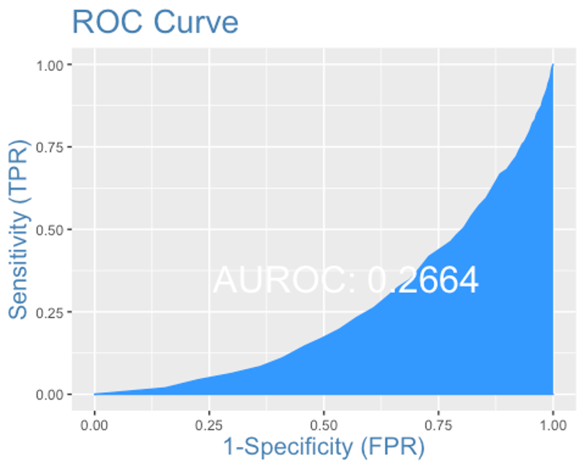
AUC는 0.266로 형편없는 성능이 나왔다.
앙상블
- 앙상블 분석을 해보자.
– 데이터는 scaled_train_ROSE, scaled_test데이터를 사용하자.
– 먼저 필요한 패키지들을 불러오자.
library(caretEnsemble)
##
## Attaching package: 'caretEnsemble'
## The following object is masked from 'package:ggplot2':
##
##     autoplot
library(caTools)
library(mlr)
## Loading required package: ParamHelpers
## Warning message: 'mlr' is in 'maintenance-only' mode since July 2019.
## Future development will only happen in 'mlr3'
## (<https://mlr3.mlr-org.com>). Due to the focus on 'mlr3' there might be
## uncaught bugs meanwhile in {mlr} - please consider switching.
##
## Attaching package: 'mlr'
## The following object is masked _by_ '.GlobalEnv':
##
##     f1
## The following object is masked from 'package:e1071':
##
##     impute
## The following object is masked from 'package:ROCR':
##
##     performance
## The following object is masked from 'package:caret':
##
##     train
library(HDclassif)
library(gbm)
## Loaded gbm 2.1.8
library(mboost)
## Loading required package: parallel
## Loading required package: stabs
##
## Attaching package: 'stabs'
## The following object is masked from 'package:mlr':
##
##     subsample
##
## Attaching package: 'mboost'
## The following object is masked from 'package:partykit':
##
##     varimp
## The following object is masked from 'package:ggplot2':
##
##     %+%
## The following objects are masked from 'package:psych':
##
##     %+%, AUC
## The following object is masked from 'package:pastecs':
##
## extract- 10-fold 교차검증을 사용하자.
control <- trainControl(method = 'cv', number = 10,
                        savePredictions = 'final',
                        classProbs = TRUE,
summaryFunction = twoClassSummary)- 모형을 학습시키자. rpart, MARS, knn을 사용해 보자.
set.seed(321)
levels(scaled_train_ROSE$Revenue)[levels(scaled_train_ROSE$Revenue) == 'TRUE'] <- 'Yes'
levels(scaled_train_ROSE$Revenue)[levels(scaled_train_ROSE$Revenue) == 'FALSE'] <- 'No'

levels(scaled_test$Revenue)[levels(scaled_test$Revenue) == 'TRUE'] <- 'Yes'
levels(scaled_test$Revenue)[levels(scaled_test$Revenue) == 'FALSE'] <- 'No'

Models <- caretList(Revenue ~., data = scaled_train_ROSE,
                    trControl = control,
                    metric = 'ROC',
                    methodList = c('rpart', 'earth', 'knn'))
Models
## $rpart
## CART
##
## 8632 samples
##   17 predictor
##    2 classes: 'No', 'Yes'
##
## No pre-processing
## Resampling: Cross-Validated (10 fold)
## Summary of sample sizes: 7768, 7768, 7770, 7769, 7768, 7769, ...
## Resampling results across tuning parameters:
##
##   cp          ROC        Sens       Spec
##   0.01593999  0.8319226  0.9232685  0.7372222
##   0.11298640  0.8108015  0.9221244  0.6977845
##   0.54688233  0.5758940  0.9791589  0.1726292
##
## ROC was used to select the optimal model using the largest value.
## The final value used for the model was cp = 0.01593999.
##
## $earth
## Multivariate Adaptive Regression Spline
##
## 8632 samples
##   17 predictor
##    2 classes: 'No', 'Yes'
##
## No pre-processing
## Resampling: Cross-Validated (10 fold)
## Summary of sample sizes: 7768, 7768, 7770, 7769, 7768, 7769, ...
## Resampling results across tuning parameters:
##
##   nprune  ROC        Sens       Spec
##    2      0.7503215  0.9216641  0.6258612
##   14      0.9497227  0.8879915  0.8600587
##   27      0.9573285  0.8939501  0.8776347
##
## Tuning parameter 'degree' was held constant at a value of 1
## ROC was used to select the optimal model using the largest value.
## The final values used for the model were nprune = 27 and degree = 1.
##
## $knn
## k-Nearest Neighbors
##
## 8632 samples
##   17 predictor
##    2 classes: 'No', 'Yes'
##
## No pre-processing
## Resampling: Cross-Validated (10 fold)
## Summary of sample sizes: 7768, 7768, 7770, 7769, 7768, 7769, ...
## Resampling results across tuning parameters:
##
##   k  ROC        Sens       Spec
##   5  0.8472500  0.6852954  0.8347429
##   7  0.8248064  0.6788734  0.8124727
##   9  0.8100880  0.6745229  0.7932601
##
## ROC was used to select the optimal model using the largest value.
## The final value used for the model was k = 5.
##
## attr(,"class")
## [1] "caretList"
scaled_train_ROSE의 Revenue변수의 levels 이름이 TRUE와 FALSE면 오류가 나서 이름을 Yes와 No로 바꿔줬다.
- 데이터 프레임 안의 테스트 세트에서 ’Yes’에 관한 예측값을 얻어오자.
model_preds <- lapply(Models, predict, newdata = scaled_test, type = 'prob')
model_preds <- lapply(model_preds, function(x) x[, 'Yes'])
model_preds <- data.frame(model_preds)- stack으로 로지스틱 회귀 모형을 쌓아보자.
stack <- caretStack(Models, method = 'glm', metric = 'ROC',
                    trControl = trainControl(
                      method = 'boot', number = 10,
                      savePredictions = 'final',
                      classProbs = TRUE,
                      summaryFunction = twoClassSummary
                    ))
summary(stack)
##
## Call:
## NULL
##
## Deviance Residuals:
##     Min       1Q   Median       3Q      Max
## -3.0708  -0.2660  -0.1108   0.2792   2.9108
##
## Coefficients:
##             Estimate Std. Error z value Pr(>|z|)
## (Intercept)   4.8122     0.1170  41.130  < 2e-16 ***
## rpart        -0.6179     0.1676  -3.688 0.000226 ***
## earth        -5.5790     0.1614 -34.556  < 2e-16 ***
## knn          -3.8415     0.1482 -25.924  < 2e-16 ***
## ---
## Signif. codes:  0 '***' 0.001 '**' 0.01 '*' 0.05 '.' 0.1 ' ' 1
##
## (Dispersion parameter for binomial family taken to be 1)
##
##     Null deviance: 11965.3  on 8631  degrees of freedom
## Residual deviance:  3983.7  on 8628  degrees of freedom
## AIC: 3991.7
##
## Number of Fisher Scoring iterations: 6
모형의 계수가 모두 유의하다.
- 앙상블에 사용된 학습자의 각 예측 결과를 비교해보자.
prob <- 1 - predict(stack, newdata = scaled_test, type = 'prob')
model_preds$ensemble <- prob
colAUC(model_preds, scaled_test$Revenue)
##                rpart     earth       knn ensemble
## No vs. Yes 0.6463632 0.7198927 0.6373395 0.539174
각 모형의 AUC를 봤을 때 앙상블 모형이 오히려 단독 모형들보다 성능이 떨어진다.
- 앙상블 모형으로 confusion matrix를 만들어 보자.
class <- predict(stack, newdata = scaled_test, type = 'raw')
head(class)
## [1] Yes Yes Yes Yes Yes Yes
## Levels: No Yes
detach('package:InformationValue', unload = TRUE)
ensemble.confusion <- confusionMatrix(class, scaled_test$Revenue, positive = 'Yes')
ensemble.confusion
## Confusion Matrix and Statistics
##
##           Reference
## Prediction   No  Yes
##        No   168   75
##        Yes 2958  497
##
##                Accuracy : 0.1798
##                  95% CI : (0.1676, 0.1926)
##     No Information Rate : 0.8453
##     P-Value [Acc > NIR] : 1
##
##                   Kappa : -0.0253
##
##  Mcnemar's Test P-Value : <2e-16
##
##             Sensitivity : 0.86888
##             Specificity : 0.05374
##          Pos Pred Value : 0.14385
##          Neg Pred Value : 0.69136
##              Prevalence : 0.15468
##          Detection Rate : 0.13440
##    Detection Prevalence : 0.93429
##       Balanced Accuracy : 0.46131
##
##        'Positive' Class : Yes
##
ensemble.confusion$byClass
##          Sensitivity          Specificity       Pos Pred Value
##            0.8688811            0.0537428            0.1438495
##       Neg Pred Value            Precision               Recall
##            0.6913580            0.1438495            0.8688811
##                   F1           Prevalence       Detection Rate
##            0.2468339            0.1546782            0.1343970
## Detection Prevalence    Balanced Accuracy
##            0.9342888            0.4613120
앙상블 모형의 성능은 Accuracy : 0.180, Kappa : -0.025, F1-score : 0.247, AUC : 0.539로 지금까지 만든 다른 모형보다 성능이 떨어지는 편이다.
Conclusion
- 모든 분석이 끝났다.
- 총 6개의 모형을 만들었고, 각 모형의 평가 지표가 어떻게 나왔는지 비교해보자.
| - | MARS | KNN | SVM | Random Forest | XGBoost | Ensemble |
|---|---|---|---|---|---|---|
| Accuracy | 0.713 | 0.690 | 0.846 | 0.910 | 0.180 | 0.180 |
| F1-score | 0.468 | 0.298 | 0.177 | 0.676 | 0.236 | 0.247 |
| AUC | 0.860 | 0.645 | 0.759 | 0.937 | 0.266 | 0.539 |
6개의 모형 중 랜덤포레스트 모형이 성능이 월등히 좋은 것으로 나타났다.
다만 Accuracy가 0.909로 매우 높은 수치를 보인 것에 비해 F1-score가 0.676으로 비교적 낮은 수치를 보이고 있는데, 이는 Accuracy가 전체 데이터에서 올바르게 분류한 데이터의 비율로 bias에 관한 단점을 가지기 때문이다.
랜덤 포레스트 모형의 Confusion Matrix를 보면 아래의 표와 같다.
| - | Reference | Reference |
|---|---|---|
| Prediction | FALSE | TRUE |
| FALSE | 3020 | 226 |
| TRUE | 106 | 346 |
Accuracy : 전체 데이터에서 올바르게 분류한 데이터의 비율은 (3020 + 346) / (3020 + 226 + 106 + 346) = 0.910
Precision : TRUE로 예측한 것 중에서 실제로 TRUE인 데이터의 비율은 346 / (106 + 346) = 0.765
Recall : 실제 TRUE인 값 중 TRUE로 예측한 비율은 226 / (226 + 346) = 0.395
여기서 Precision과 Recall이 둘 다 높으면 가장 좋은 방법이겠지만, 이 둘은 반비례하는 경향이 있다. 이를 보완하기 위해 이 둘의 조화평균을 사용하는 F1-score를 사용한다.