AlexNet
Abstract
ImageNet LSVRC-2010 대회에서 1000개의 클래스의 120만 고해상도 이미지를 분류하기 위해 대규모 deep convolution network를 훈련했다.
신경망은 6천만 개의 파라미터와 65만개의 뉴런과 5개의 convolution layer(몇몇은 3개의 max pooling) 그리고 3개의 fc layer로 이루어져 있으며 마지막에는 softmax로 분류하는 구조로 이루어져있다.
Introduction
현재 object recognition에서 머신러닝 기법을 필수적으로 사용하고 있다.
상대적으로 작은 데이터 셋으로는 간단한 object recognition에서 잘 사용할 수 있었는데, 실제 데이터셋은 많은 변동성이 포함되어있기에 이를 인식하기 위해서는 더 큰 데이터 셋이 필요하다
수백만개 이미지에서 수천 개의 객체를 학습하기 위해서는 더 큰 학습 능력을 가진 모델이 필요하다. CNN의 용량은 깊이와 폭을 제어할 수 있고, 이미지의 특성에 대해 정확한 추정이 가능하다. 하지만, CNN은 고해상도 이미지에 사용하기에 비용이 많이 들기에, 최신 GPU를 사용하여 2D 합성곱의 최적화 구현과 훈련을 한다. 또한, 과적합 방지를 위해 여러 기술들을 사용하였다.
ReLU Nonlinearity
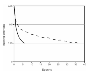
깊은 CNN에서 기존의 tanh 함수보다 ReLU를 사용하는 것이 최적화 속도가 빠르기 때문에,
ReLU를 사용한다.
Training on Multiple GPUs
하나의 GTX 580 GPU는 3GB의 메모리를 가지며, 이는 네트워크가 학습할 수 있는 최대 사이즈를 제한한다. 이것은 120만의 학습 샘플들을 학습시키기에는 충분하지만, 하나의 GPU에 학습시키는 것은 너무 크다. 따라서, 우리는 두 개의 GPU를 나눠서 사용하는데 최신 GPU들은 다른 GPU의 메모리를 직접 읽고 쓸 수 있어서 병렬 처리에 적합하다.
Local Response Normalization
ReLU 자체는 정규화가 필요하지 않지만, 특정 필터의 한 픽셀의 가중치가 높으면 주변 픽셀이 영향을 받을 수 있기에 이 논문에서는 특정 계층에 대해 local response normalization을 사용한다. (지금은 거의 사용하지 않음. 대신 Batch normalization 사용)
따라서, LRN은 Lateral inhibition과 같은 효과를 줌으로써 일반화 하였고, top1, 5의 오류율을 1.4, 1.2% 줄이는 효과가 나타났다. 또한, CIFAR - 10 데이터 셋으로 검증하여, 4층 CNN은 정규화가 없을 때 13% 정규화를 적용했을 떄는 11%의 오류율을 보였다.
Lateral inhibition : 강한 자극이 주변에 약한 자극으로 전달되는 것을 막는 효과
논문에서는 첫번째와 두번째 conv layer에서 사용했다고 나옴
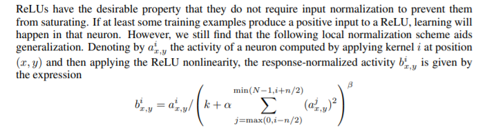
: LRN한 Activation 결과
: Activation 결과
: 현재 filter
: 고려해야 하는 filter 개수
: 총 filter 개수
: Hyper parameter
Overlapping Pooling
CNN의 풀링 레이어는 동일한 커널 맵에서 근접한 이웃 뉴런의 ouput을 저장(요약)하는데, 기존의 풀링 유닛들은 중복되는 이웃의 정보를 저장하지 못했다. 또한, 기존에는 풀링 유닛이 z*z를 사용할 때 s=z 방식을 사용했는데, s < z 로 설정하는 것으로 중복되는 풀링을 얻을 수 있었다. 이를 통해 Overffiting의 가능성을 줄일 수 있었다고 한다
Overall Architecture
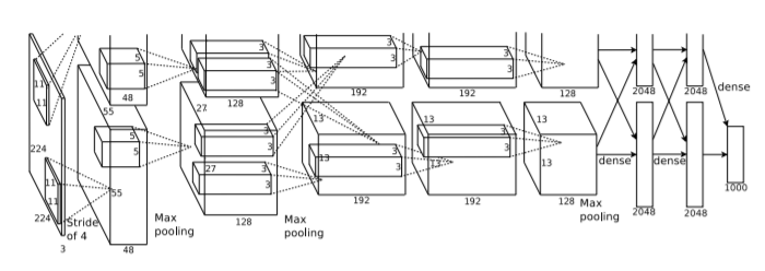
전체적인 구조를 다시 보면 8개의 later로 이루어져 있으며, 5개의 합성곱 층과 3개의 완전연결층으로 이루어져 있다. 마지막 층은 sofxmax를 통해 1000개의 분류 라벨을 뽑아낸다.
이 신경망은 다항 로지스틱 회귀를 최대화한다. 즉, 올바른 라벨의 로그 확률 예측을 최대화 한다
| layer | input | filter | stride | padding | activation | output |
|---|---|---|---|---|---|---|
| 1 conv | 227 x 227 x 3 | 11 x 11 x 3 x 96 | 4 | 0 | ReLU | 55 x 55 x 96 |
| 1 maxpool | 55 x 55 x 96 | 3 x 3 | 2 | 27 x 27 x 96 | ||
| 2 conv | 27 x 27 x 96 | 5 x 5 x 48 x 256 | 1 | 2 | ReLU | 27 x 27 x 256 |
| 2 maxpool | 27 x 27 x 256 | 3 x 3 | 2 | 13 x 13 x 256 | ||
| 3 conv | 13 x 13 x 256 | 3 x 3 x 256 x 384 | 1 | 1 | ReLU | 13 x 13 x 384 |
| 4 conv | 13 x 13 x 384 | 3 x 3 x 192 x 384 | 1 | 1 | ReLU | 13 x 13 x 384 |
| 5 conv | 13 x 13 x 384 | 3 x 3 x 192 x 256 | 1 | 1 | ReLU | 13 x 13 x 256 |
| 5 maxpool | 13 x 13 x 256 | 3 x 3 | 2 | 6 x 6 x 256 | ||
| 6 fc | 6 x 6 x 256 | ReLU | 9216 → 4096 | |||
| 7 fc | 4096 | ReLU | 4096 → 4096 | |||
| 8 fc | 1000 | softmax | 1000 |
Ovefitting 관리
- data augementation
- overfitting을 줄이기 위해 data augementation을 사용했고, 이는 GPU에서 학습이 진행되는 동안 CPU에서 진행하여 효율적.
- 첫 번째 방법은 256256 이미지에서 무작위로 227227 patch를 만들고 이를 수평 반사 후 추출하여 학습에 사용했다. 각 코너의 패치와 중앙의 패치 그리고 이들을 뒤집은 것을 포함해 총 10개의 패치를 만들어 softmax 레이어를 통과시켜 예측을 하였다.
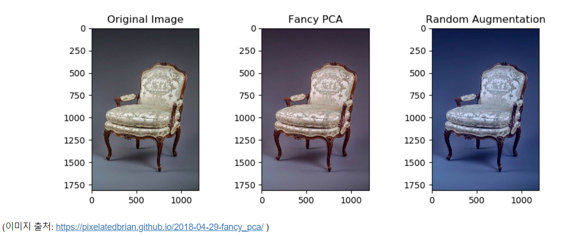
- 두 번째 방법은 PCA를 사용하여 RGB 픽셀들의 균형을 변경하는 방법인데, 평균이 0, 표준편차가 1인 정규분포에서 얻은 랜덤 변수와 PCA를 통해 나온 주성분들을 곱하여 각 이미지에 추가함으로써 증강하였다.
- Dropout
- 다양한 모델의 예측을 결합하는 것은 테스트 에러를 줄이는 좋은 방법이지만, 훈련하는데 수 일이 걸리는 모델, 비용이 많이 드는 모델의 경우에는 적합하지 않다
- 이러한 경우에 효과적으로 모델의 예측을 결합하는 방법인 dropout을 사용하여 몇몇의 뉴런을 죽이는 방법으로 뉴런의 복잡한 공동 적응을 감소시킨다.
- 처음 두 개의 fc layer에서 Dropout을 0.5로 사용하여 일부 뉴런을 죽이는 방법을 사용함으로써 overfitting을 관리하였다.
Details of learning
저자는 SGD optimizer를 사용하며 배치 사이즈는 128, weight_decay는 0.0005, 모멘텀을 0.9 로 두어 훈련을 진행하였다. 저자는 적은 양의 weight_decay가 모델 학습하는데 있어서 중요하다는 것을 찾아냈고, 단순한 정규화가 아닌 모델의 training error를 감소시킨다고 하였다.
또한, 각 layer의 weight를 평균이 0 표준편차가 0.01인 정규분포로 초기화하였으며, 2,4,5번째의 convolution layer와 fc layer에서 bias를 1로 초기화 하였다고 한다. 이러한 초기화는 ReLU에 양의 입력을 제공함으로써 학습의 초기 단계를 가속화 한다. 또한, 상수 0으로 나머지 층에서 bias를 초기화하였다.
모든 층에서 동일한 학습률을 적용했고, 훈련하는 동안 수동으로 조정했다. 이 체험은 검증 에러가 현재 학습 속도에서 향상되지 않을 때 learning rate를 10으로 나누는 방식을 사용한다.
Implement
import numpy as np
import matplotlib.pyplot as plt
import torch
import torch.nn as nn
import torch.optim as optim
import torchvision
from torchvision import datasets, transforms
from torch.nn.modules.pooling import MaxPool2d
from torch.nn.modules.normalization import LocalResponseNorm
devices = torch.device('cuda:0' if torch.cuda.is_available() else 'cpu')
print(devices)

transform = transforms.Compose([transforms.Resize(256),
                                transforms.RandomCrop(227),
                                transforms.ToTensor(),
                                # transforms.RandomHorizontalFlip(1),
                                transforms.Normalize((0.5,0.5,0.5),(0.5,0.5,0.5)),

])

ci_train = datasets.CIFAR10('~/data/', train=True, transform=transform,download=True)
ci_test = datasets.CIFAR10('~/data/', train=True, transform=transform,download=True)
print("ci_train:\n", ci_train,'\n')
print("ci_test:\n", ci_test,'\n')

batch_size = 256
train_iter = torch.utils.data.DataLoader(ci_train, batch_size=batch_size, shuffle=False, num_workers=1)
test_iter = torch.utils.data.DataLoader(ci_train, batch_size=batch_size, shuffle=True, num_workers=1)

class AlexNet(nn.Module):
  def __init__(self, input_size=227, num_classes = 10):
    super(AlexNet, self).__init__()

  # Convolution layer 정의
    self.layers = nn.Sequential(
        # 1 conv
        nn.Conv2d(in_channels=3,out_channels=96,kernel_size=11,stride=4,padding=0),
        nn.ReLU(inplace=True),
        nn.LocalResponseNorm(size =5, alpha=0.0001, beta=0.75, k=2),
        nn.MaxPool2d(kernel_size=3,stride=2),

        # 2 conv
        nn.Conv2d(in_channels=96, out_channels=256,kernel_size=5,stride=1,padding=2),
        nn.ReLU(inplace=True),
        nn.LocalResponseNorm(size=5, alpha=0.0001, beta=0.75, k=2),
        nn.MaxPool2d(kernel_size=3,stride=2),

        # 3 conv
        nn.Conv2d(in_channels=256, out_channels=384, kernel_size=3,stride=1,padding=1),
        nn.ReLU(inplace=True),


        # 4 conv
        nn.Conv2d(in_channels=384, out_channels=384, kernel_size=3,stride=1,padding=1),
        nn.ReLU(inplace=True),

        # 5 conv
        nn.Conv2d(in_channels=384, out_channels=256, kernel_size=3,stride=1,padding=1),
        nn.ReLU(inplace=True),
        nn.MaxPool2d(kernel_size=3, stride=2)
    )

    self.fclayer = nn.Sequential(
        # 6 fc layer
        nn.Dropout(0.5),
        nn.Linear(6*6*256, 4096),
        nn.ReLU(inplace=True),


        # 7 fc layer
        nn.Dropout(0.5),
        nn.Linear(4096,4096),
        nn.ReLU(inplace=True),


        # 8 fc layer
        nn.Linear(4096,num_classes)
    )

    # 표준화 및 bias 초기화
    for layer in self.layers:
      if isinstance(layer, nn.Conv2d):
        nn.init.normal_(layer.weight, mean=0, std=0.01)
        nn.init.constant_(layer.bias,0)

    #nn.init.constant_(self.layers[4].bias,1)
    #nn.init.constant_(self.layers[10].bias,0.8)
    #nn.init.constant_(self.layers[12].bias,0.6)

  def forward(self, train):
    output = self.layers(train)
    output = torch.flatten(output,1)
    output = self.fclayer(output)

    return output

alexnet = AlexNet(227,10)
alexnet.to(devices)

optimizer = optim.SGD(alexnet.parameters(),lr=0.01,momentum=0.9, weight_decay = 0.0005)
criterion = nn.CrossEntropyLoss().to(devices)

from tqdm.notebook import tqdm
import time

start_time = time.time()
min_loss = int(1e9)
history = []
accuracy = []

for epoch in range(20):
    epoch_loss = 0
    tk0 = tqdm(train_iter, total=len(train_iter),leave=False)
    for step, (inputs, labels) in enumerate(tk0, 0):
        inputs, labels = inputs.to(devices), labels.to(devices)
        outputs = alexnet(inputs)
        loss = criterion(outputs, labels)

        optimizer.zero_grad()
        loss.backward()
        optimizer.step()

        epoch_loss += loss.item()
        history.append(loss.item())

    class_correct = list(0. for i in range(1000))
    class_total = list(0. for i in range(1000))

    with torch.no_grad():
        for data in test_iter:
            images, labels = data
            images = images.to(devices)
            labels = labels.to(devices)
            outputs = alexnet(images)
            _, predicted = torch.max(outputs, 1)
            c = (predicted == labels).squeeze()
            for i in range(labels.size()[0]):
                label = labels[i].item()
                class_correct[label] += c[i].item()
                class_total[label] += 1

    accuracy.append(sum(class_correct) /sum(class_total)*100)
    tqdm.write("[Epoch : %d] train_loss : %.5f test_acc: %.2f" %
               (epoch +1 , epoch_loss/196, sum(class_correct) /sum(class_total)*100))

    if min_loss < epoch_loss:
      count+=1
      if count > 10:
        for g in optimizer.param_groups:
          g['lr']/=10
    else:
      min_loss = epoch_loss
      count = 0

print(time.time()-start_time)
print("Done")
Reference
https://proceedings.neurips.cc/paper/2012/file/c399862d3b9d6b76c8436e924a68c45b-Paper.pdf
