3층 신경망 구현하기
3층 신경망은 입력층은 2개, 첫 번째 은닉층은 3개, 두 번째 은닉층은 2개, 출력층은 2개의 뉴런으로 구성된다.
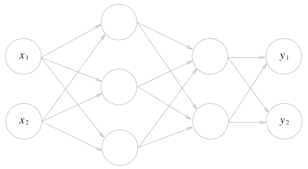
입력층에서 1층으로 신호 전달
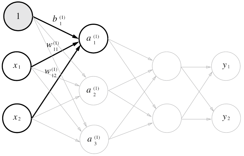
X = np.array([1.0, 0.5])
W1 = np.array([[0.1, 0.3, 0.5], [0.2, 0.4, 0.6]])
B1 = np.array([0.1, 0.2, 0.3])

print(W1.shape) # (2, 3)
print(X.shape) # (2, )
print(B1.shape) # (3, )

A1 = np.dot(X, W1) + B1
Z1 = sigmoid(A1)

print(A1) # [0.3, 0.7, 1.1]
print(Z1) # [ 0.57444252, 0.66818777, 0.75026011]
1층에서 2층으로 신호 전달
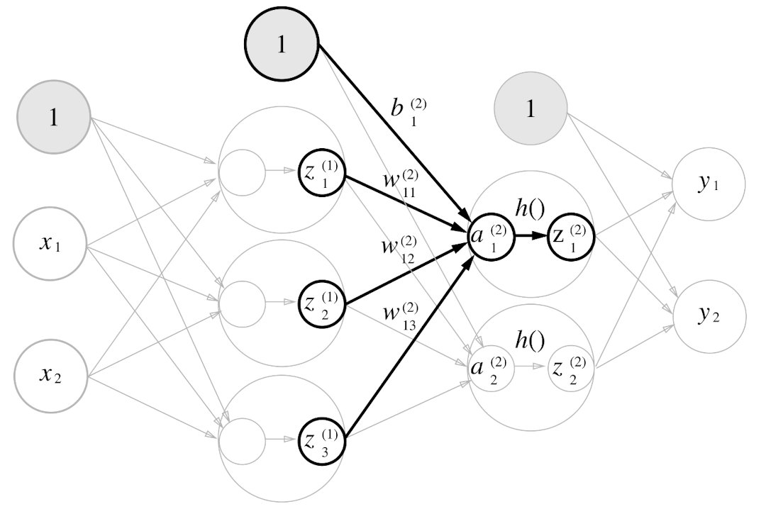
W2 = np.array([[0.1, 0.4], [0.2, 0.5], [0.3, 0.6]])
B2 = np.array([0.1, 0.2])

print(Z1.shape) # (3, )
print(W2.shape) # (3, 2)
print(B2.shape) # (2, )

A2 = np.dot(Z1, W2) + B2
Z2 = sigmoid(A2)
2층에서 출력층으로 신호 전달
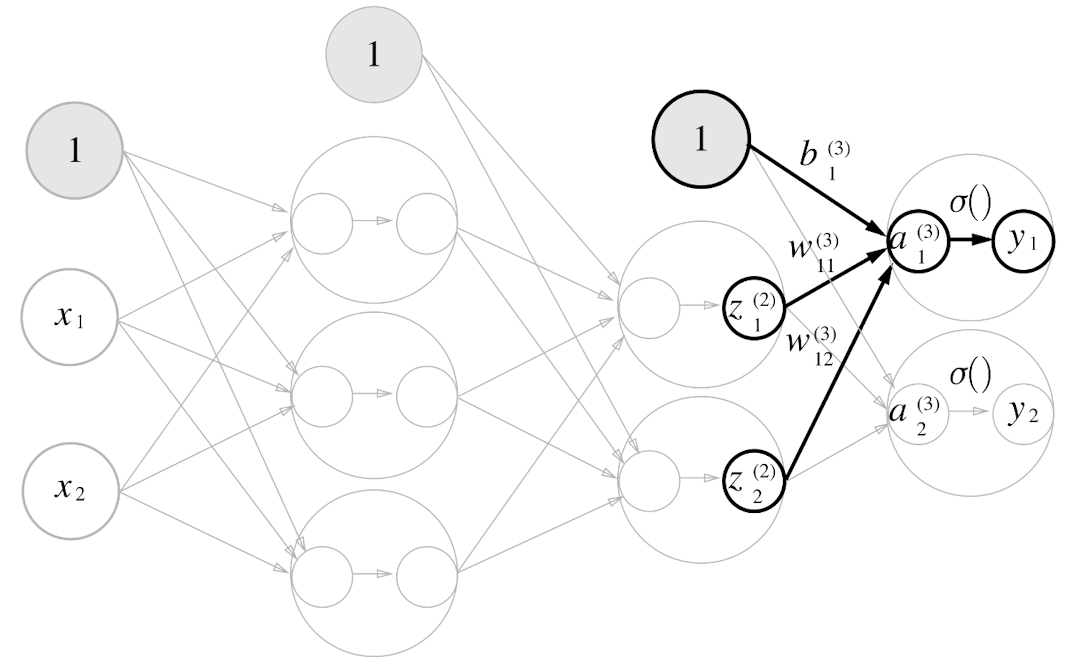
def identity_function(x):
	return x

W3 = np.array([[0.1, 0.3], [0.2, 0.4]])
B3 = np.array([0.1, 0.2])

A3 = np.dot(Z2, W3) + B3
Y = identity_function(A3)- 항등 함수 identity_function()을 정의하고, 출력층의 활성화 함수로 이용한다.
전체 구현 정리
def init_network():
	network = {}
    network['W1'] = np.array([[0.1, 0.3, 0.5], [0.2, 0.4, 0.6]])
    network['b1'] = np.array([0.1, 0.2, 0.3])
    network['W2'] = np.array([0.1, 0.4], [0.2, 0.5], [0.3, 0.6]])
    network['b2'] = np.array([0.1, 0.2])
    network['W3'] = np.array([[0.1, 0.3], [0.2, 0.4]])
    network['b3'] = np.array([0.1, 0.2])

    return network

def forward(network, x):
	W1, W2, W3 = network['W1'], network['W2'], network['W3']
    b1, b2, b3 = network['b1'], network['b2'], network['b3']

    a1 = np.dot(x, W1) + b1
    z1 = sigmoid(a1)
    a2 = np.dot(z1, W2) + b2
    z2 = sigmoid(a2)
    a3 = np.dot(z2, W3) + b3
    y = identity_function(a3)

    return y

network = init_network()
x = np.array([1.0, 0.5])
y = forward(network, x)
print(y) # [0.31682708 0.69627909]
출력층 설계하기
기계학습 문제에는 분류와 회귀가 있다.
- 분류는 데이터가 어느 클래스에 속하느냐는 문제이고, 출력층의 활성화 함수로 소프트맥스 함수를 사용한다. - - 회귀는 입력 데이터에서 수치를 예측하는 문제이고, 출력층의 활성화 함수로 항등 함수를 사용한다.
항등 함수, 소프트맥스 함수 구현하기
항등 함수
입력을 그대로 출력, 입력과 출력이 항상 같다
소프트맥스 함수
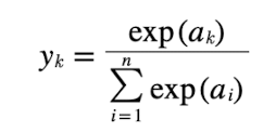
def softmax(a):
	exp_a = np.exp(a)
    sum_exp_a = np.sum(exp_a)
    y = exp_a / sum_exp_a

return y- 소프트맥스 함수는 오버플로(컴퓨터로 계산할 때 표현할 수 있는 수의 범위가 한정되어 너무 큰 값은 표현할 수 없음) 문제가 생긴다.
오버플로를 해결한 소프트맥스 함수
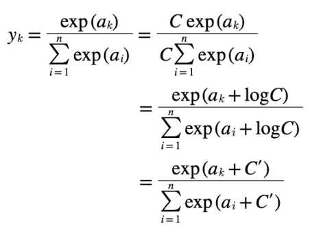 ```python
def softmax(a):
x = np.max(a)
exp_a = np.exp(a - c)
sum_exp_a = np.sum(exp_a)
y = exp_a / sum_exp_a
return y
```
```python
def softmax(a):
x = np.max(a)
exp_a = np.exp(a - c)
sum_exp_a = np.sum(exp_a)
y = exp_a / sum_exp_a
return y
```
소프트맥스 함수의 특징
- 소프트맥스 함수 출력의 총합은 1이다. 확률과 비슷하다.
- 소프트맥스 함수를 적용해도 각 원소의 대소 관계는 변하지 않는다. → 지수 함수 y = exp(x)가 단조 증가 함수이기 때문이다.
- 출력층의 소프트맥스 함수는 생략 가능
손글씨 숫자 인식
신경망에서는 훈련 데이터를 사용해 가중치 매개변수를 학습하고, 추론 단계에서는 앞서 학습한 매개변수를 사용하여 입력 데이터를 분류한다.
MNIST 데이터셋
- MNIST 데이터 가져오기
import sys, os
sys.path.append(os.pardir)
from dataset.mnist import load_mnist

(x_train, t_train), (x_test, t_test) = \
	load_mnist(flatten=True, normalize=False)

print(x_train.shape) # (60000, 784)
print(t_train.shape) # (60000, )
print(x_test.shape)  # (10000, 784)
print(t_test.shape). # (10000, )- load_mnist() 함수로 MNIST 데이터를 가져온다. load_mnist() 함수의 인수로 normalize, flatten, one_hot_label bool값으로 설정이 가능하다.
normalize: 입력 이미지의 픽셀 값을 0.0~1.0 사이의 값으로 정규화할지 정한다. False → 입력 이미지의 픽셀 원래 값 그대로 0~255 사이의 값 유지
flatten: 입력 이미지를 1차원 배열로 만들지 정한다, False → 입력 이미지를 1x28x28의 3차원 배열로 저장, True → 784개의 원소로 이루어진 1차원 배열로 저장
one_hot_label: 레이블을 원-핫 인코딩 형태로 저장할 지를 정한다, False → 숫자 형태의 레이블을 저장, True → 레이블을 원-핫 인코딩하여 저장 - MNIST 이미지 불러오기
import sys, os
sys.path.append(os.pardir)
import numpy as np
from dataset.mnist import load_mnist
from PIL import Image

def img_show(img):
	pil_img = Image.fromarray(np.uint8(img))
    pil_img.show()

(x_train, t_train), (x_test, t_test) = \
	load_mnist(flatten=True, normalize=False)

img = x_train[0]
label = t_train[0]
print(label) # 5

print(img.shape) 			# (784, )
img = img.reshape(28, 28)   # 원래 이미지 모양으로 변형
print(img.shape)			# (28, 28)

img_show(img)
읽어들인 이미지가 1차원 넘파이 배열로 저장되어 있어서 reshape() 메서드로 28x28 크기로 다시 변형한다.
신경망의 추론 처리
- 입력층 뉴런은 이미지의 크기인 28x28=784개의 뉴런으로 되어있고, 출력층 뉴런은 10개이고, 은닉층은 두 개로 구성되어 있는데 첫번째는 50개, 두번째는 100개이다.
def get_data():
	(x_train, t_train), (x_test, t_test) = \
    	load_mnist(normalize=True, flatten=True, one_hot_label=False)
    return x_test, t_test

def init_network():
	with open("sample_weight.pkl", 'rb') as f:
    	network = pickle.load(f)

    return network

def predict(network, x):
	W1, W2, W3 = network['W1'], network['W2'], network['W3']
    b1, b2, b3 = network['b1'], network['b2'], network['b3']

    a1 = np.dot(x, W1) + b1
    Z1 = sigmoid(a1)
    a2 = np.dot(z1, W2) + b2
    Z2 = sigmoid(a2)
    a3 = np.dot(z2, W3) + b3
    y = softmax(a3)

    return y
init_network() 함수에서는 파일에 저장된 학습된 가중치 매개변수를 읽는다.
정확도 평가
x, t = get_data()
network = init_network()

accuracy_cnt = 0
for i in range(len(x)):
	y = predict(network, x[i])
    p = np.argmax(y)
    if p == t[i]:
    	accuracy_cnt += 1

print("Accuracy:" + str(float(accuracy_cnt) / len(x)))
데이터를 특정 범위로 변환하는 처리를 정규화라고 하고, 신경망의 입력 데이터에 특정 변환을 가하는 것을 전처리라고 한다.
배치 처리
x, t = get_data()
network = init_network()

batch_size = 100
accruracy_cnt = 0

for i in range(0, len(x), batch_size):
	x_batch = x[i:i+batch_size]
    y_batch = predict(network, x_batch)
    p = np.argmax(y_batch, axis=1)
    accuracy_cnt += np.sum(p == t[i:i+batch_size])

print("Accuracy:" + str(float(accuracy_cnt) / len(x)))- np.argmax(): 최댓값의 인덱스를 가져온다.
