들어가기에 앞서서 코딩은 kaggle에서 진행하였다.

데이터셋 준비

먼저 캐글에서 노트북을 생성하면 자동으로 아래의 코드가 생성이 된다.

# This Python 3 environment comes with many helpful analytics libraries installed
# It is defined by the kaggle/python Docker image: https://github.com/kaggle/docker-python
# For example, here's several helpful packages to load

import numpy as np # linear algebra
import pandas as pd # data processing, CSV file I/O (e.g. pd.read_csv)

# Input data files are available in the read-only "../input/" directory
# For example, running this (by clicking run or pressing Shift+Enter) will list all files under the input directory

import os
for dirname, _, filenames in os.walk('/kaggle/input'):
    for filename in filenames:
        print(os.path.join(dirname, filename))

# You can write up to 20GB to the current directory (/kaggle/working/) that gets preserved as output when you create a version using "Save & Run All" 
# You can also write temporary files to /kaggle/temp/, but they won't be saved outside of the current session

그 후 우리는 사이킷런에서 제공하는 데이터셋 중 유명한 보스턴 주택 가격 데이터 세트를 로드하고, 이를 DataFrame으로 생성하는 코드를 작성했다.

from sklearn.datasets import load_boston

boston = load_boston()
bostonDF = pd.DataFrame(boston.data, columns=boston.feature_names)
bostonDF['PRICE'] = boston.target
print(bostonDF.shape)
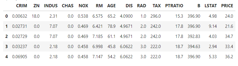
bostonDF.head()

그 중 PRICE라는 특성은 우리가 예측하려고 하는 주택의 가격이기 때문에, boston.target으로 지정을 해주었다.
그런다음 코드를 실행해주면 아래의 그림과같이 DataFrame으로 잘 생성이 된 것을 볼 수 있다.

경사하강법을 통한 값을 계산하는 함수 생성

먼저 이 상황에서는 학습에 적용한 특성을 먼저 2가지로 추렸는데, RM(방의 개수)와 LSTAT(하위계층 비율) 이 두가지의 특성만을 가지고 학습을 진행하였다.
이때 w1은 RM특성의 가중치값,
w2는 LSTAT특성의 가중치값으로 설정하였다.
먼저 함수를 정의해준다.

def get_update_weights_value(bias, w1, w2, rm, lstat, target, learning_rate=0.01):
    
    # 데이터 건수
    N = len(target)
    # 예측 값. 
    predicted = w1 * rm + w2*lstat + bias
    # 실제값과 예측값의 차이 
    diff = target - predicted
    # bias 를 array 기반으로 구하기 위해서 설정. 
    bias_factors = np.ones((N,))

여기서 target은 PRICE이고, 학습률의 기본값은 0.01로 설정해 주었다.
bias_factors를 np.ones를 이용해 넘파이 배열의 형태로 생성해 준 이유는 bias를 배열 기반으로 구하기 위해 설정해주었다.

그런다음 update연산을 수행해준다.

 # weight와 bias를 얼마나 update할 것인지를 계산.  
 w1_update = -(2/N)*learning_rate*(np.dot(rm.T, diff))
 w2_update = -(2/N)*learning_rate*(np.dot(lstat.T, diff))
 bias_update = -(2/N)*learning_rate*(np.dot(bias_factors.T, diff))
    
 # Mean Squared Error값을 계산. 
 mse_loss = np.mean(np.square(diff))
    
 # weight와 bias가 update되어야 할 값과 Mean Squared Error 값을 반환. 
 return bias_update, w1_update, w2_update, mse_loss

지금 현재 diff값은 배열형태이기 때문에 (위에서 입력되는 rm, lstat, target모두 array가 입력되기 때문) np.dat을 이용해서 행렬의 곱셈을 수행해준다.
그후 diff값들을 제곱해준뒤 평균을 내서 mse_loss값을 설정해주고, bias, w1, w2의 업데이트 값과 mse_loss값을 리턴해준다.

경사하강법을 적용하는 함수 생성

그 다음은 특성들과 타겟 array를 입력받아 특성 epochs 수만큼 반복적으로 가중치와 Bias를 업데이트 하는 함수를 작성해야한다.

def gradient_descent(features, target, iter_epochs=1000, verbose=True):
    # w1, w2는 numpy array 연산을 위해 1차원 array로 변환하되 초기 값은 0으로 설정
    # bias도 1차원 array로 변환하되 초기 값은 1로 설정. 
    w1 = np.zeros((1,))
    w2 = np.zeros((1,))
    bias = np.zeros((1, ))
    print('최초 w1, w2, bias:', w1, w2, bias)
    
    learning_rate = 0.01
    rm = features[:, 0]
    lstat = features[:, 1]

여기서 features에는 rm과 lstat 두개의 값이 들어가고, target에는 PRICE 특성이 들어간다. w1, w2는 초기값이 0인 1차원 array로 설정하고, bias값은 초기값이 1인 1차원 array로 설정한다.

그 후 learning_rate와 RM, LSTAT 특성을 지정해준다.
위와 같은 형태로 코드를 작성한 이유는 후에 작성할 코드에서 호출시에 numpy array형태로 RM과, LSTAT으로 된 2차원 feature가 입력되기 때문이다.

그 후 아래의 코드에서 iter_epoch 수만큼 반복하면서 업데이트를 수행하는 코드를 작성한다. 그후 값을 출력하는 코드또한 작성해준다.

for i in range(iter_epochs):
        # weight/bias update 값 계산 
        bias_update, w1_update, w2_update, loss = get_update_weights_value(bias, w1, w2, rm, lstat, target, learning_rate)
        # weight/bias의 update 적용. 
        w1 = w1 - w1_update
        w2 = w2 - w2_update
        bias = bias - bias_update
        if verbose:
            print('Epoch:', i+1,'/', iter_epochs)
            print('w1:', w1, 'w2:', w2, 'bias:', bias, 'loss:', loss)

경사하강법을 적용한 뒤 Price예측

먼저 신경망 모델은 데이터를 정규화/표준화 작업을 통해 미리 개별 feature값을 0~1사이 값으로 변환 후 학습을 적용하여야 한다. 이를 위해 사이킷런의 MinMaxScaler를 이용하였다.

from sklearn.preprocessing import MinMaxScaler

scaler = MinMaxScaler()
scaled_features = scaler.fit_transform(bostonDF[['RM', 'LSTAT']])

w1, w2, bias = gradient_descent(scaled_features, bostonDF['PRICE'].values, iter_epochs=5000, verbose=True)
print('##### 최종 w1, w2, bias #######')
print(w1, w2, bias)

그런 뒤 계산된 가충치값과 Bias를 이용해 Price를 예측한다. 예측 feature역시 0~1 사이의 값을 이용한다.

predicted = scaled_features[:, 0]*w1 + scaled_features[:, 1]*w2 + bias
bostonDF['PREDICTED_PRICE'] = predicted
bostonDF.head(10)

위의 코드를 모두실행하면 다음과 같은 결과가 나타난다.

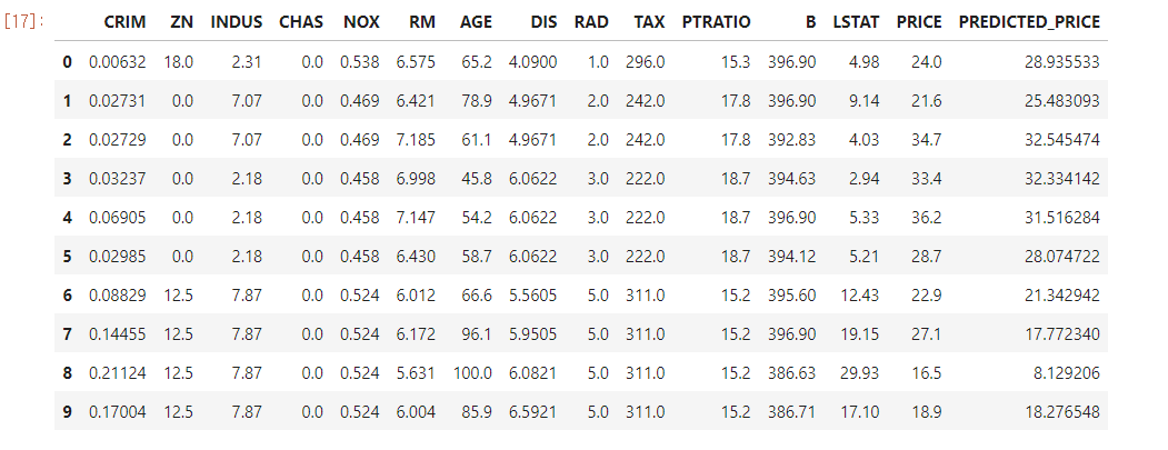
여기서 PREDICTED_PRICE가 예측을 한 값이다. 결과를 보면 실제 가격과 어느정도 들어맞는것을 볼 수 있다.