Week 9-1. Image Homograph and Stitching
1. Image Stitching
motivation: panorama
1. Capture multiple image from different viewpoints
2. Stitch them together into a virtual wide-angle image
How?
Translate one image relative to another- not enough- use homographies
2. Projective Transformation (Homography)
Classification of 2D Transformation
warp하려면 어떤 transformation이 필요한가
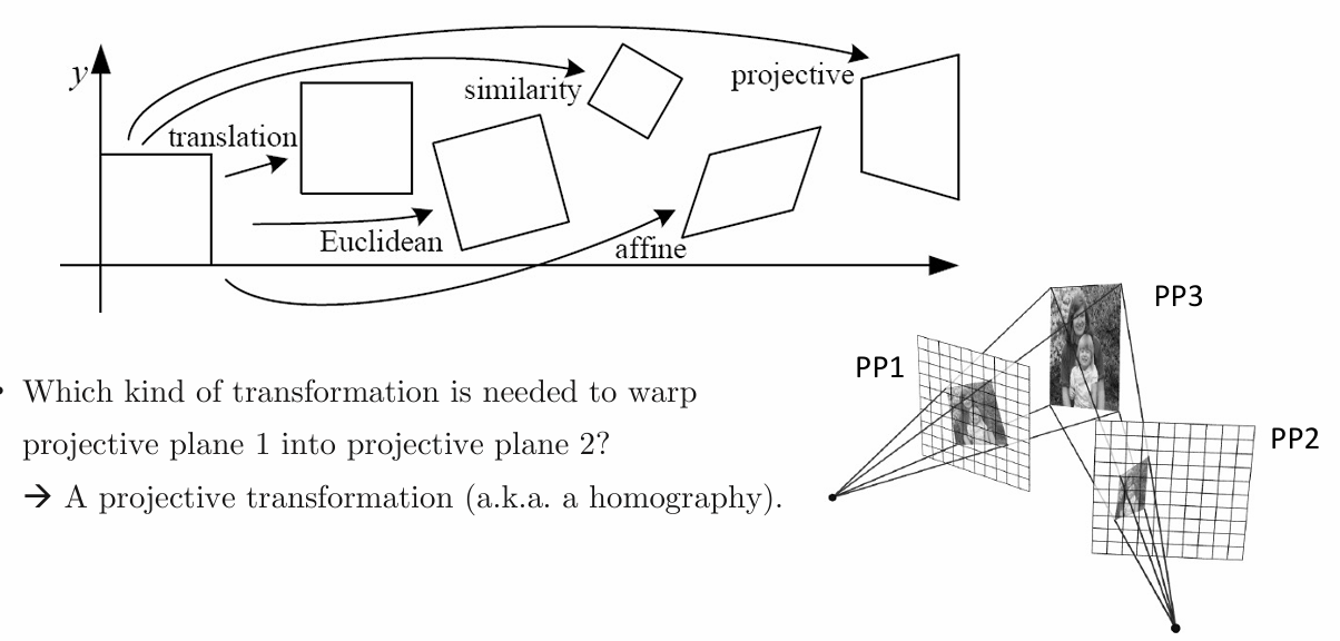
Projective Transformation (Homography)
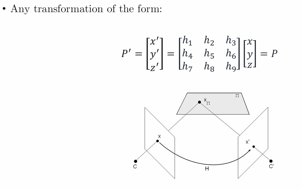
scale만 정의 가능, 이면 8 free parameters
origin이 origin map할 필요 없음, parallel line이 map하고 평행할 필요 없음, lines map to lines
closed under composition
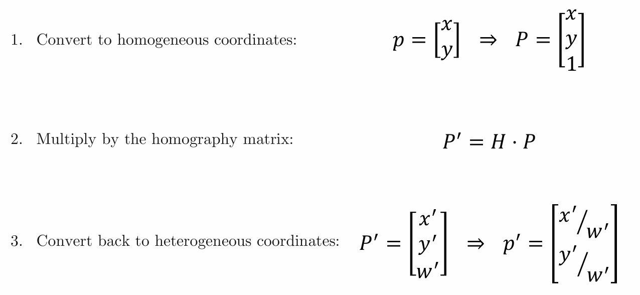
- applying a Homography
homogeneous coordinates 좌표
homography matrix 곱함
heterogeneous coordinates로 돌아감
3. Computing Homograph
Determining the Homography Matrix
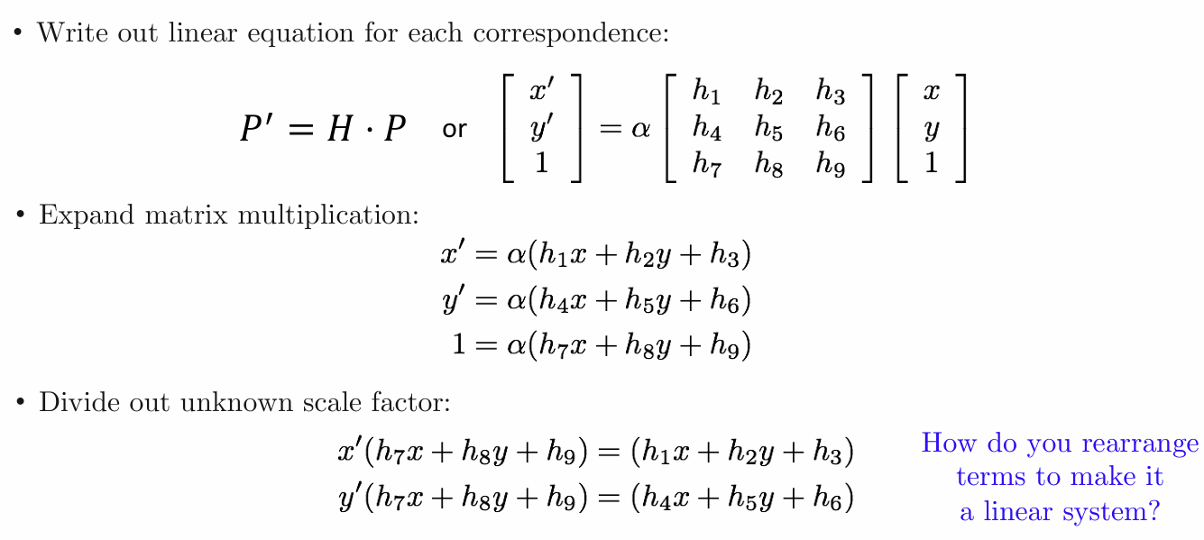
맨 아래 식을 위에 대입, re-arrange terms 나옴
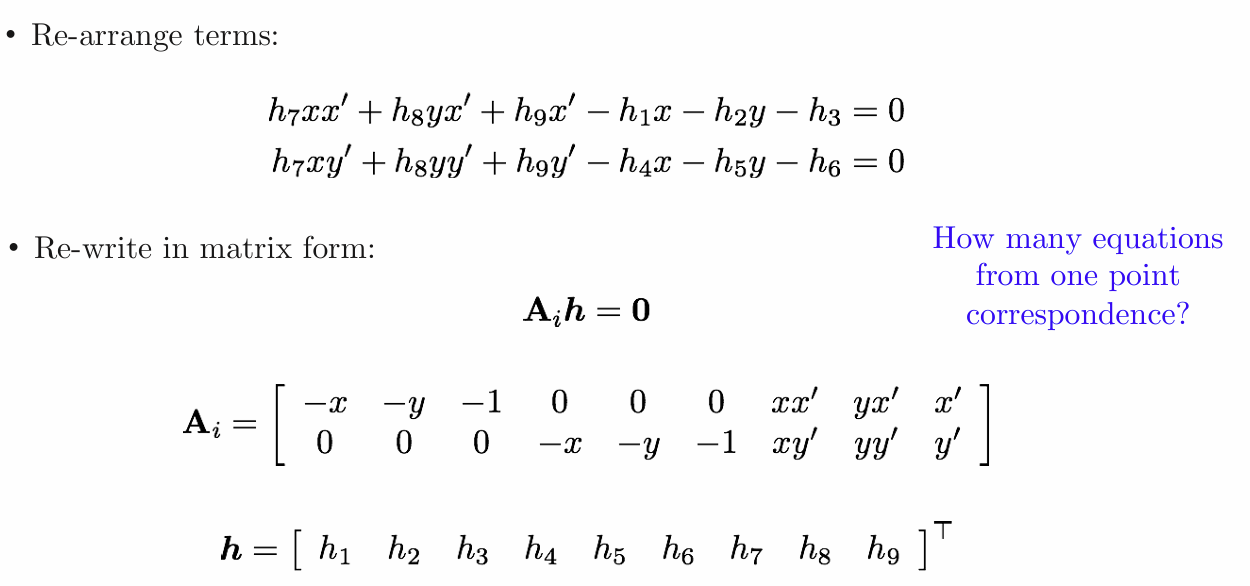
여러 점 대응관계에서 constraints 쌓기, 식은 다음페이지
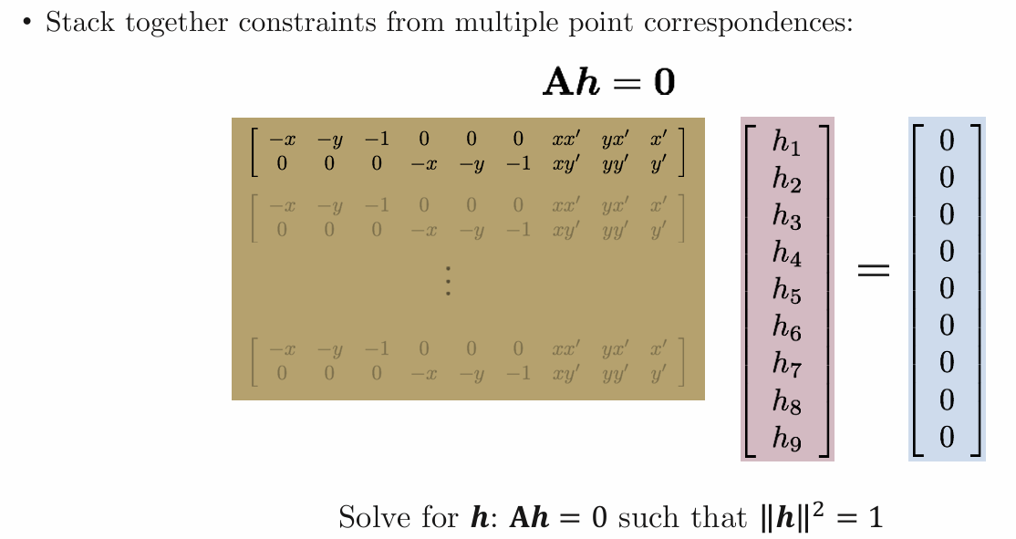
Constrained Least Squares
least squares problem
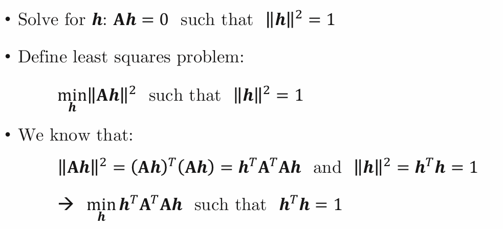
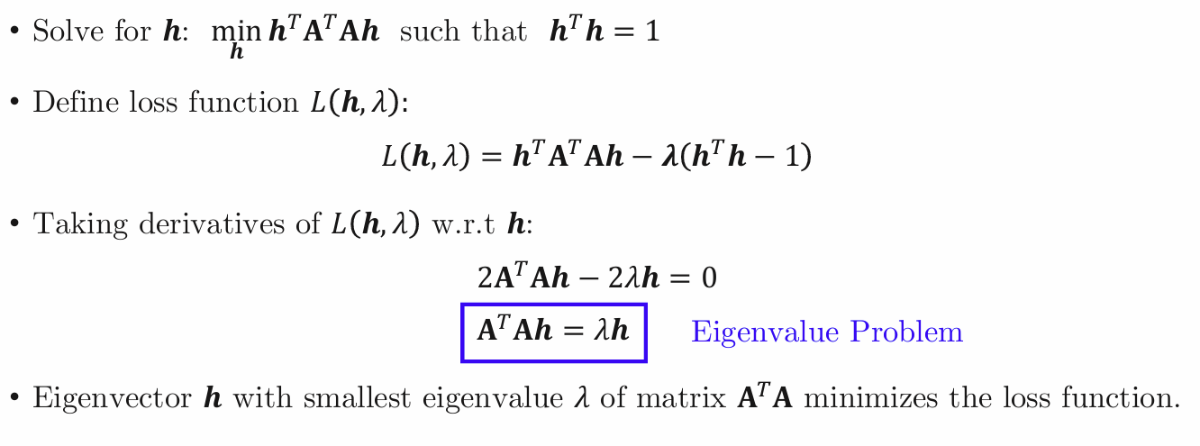
loss function = Ah^2 - \eigenvalue * (h^2 -1)
미분 = 0 eigenvalue problem; 의 최소 eigen value인 Eigenvector h가 답, loss function 최소화
4. Image Warping
Given a coordinate transform and a source image f(x,y),
transformed image g(x',y') = f(T(x,y)) 어떻게 compute?
Forward vs Inverse Warping
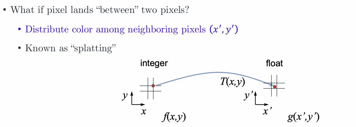
Forward Warping
send each pixel f(x,y) to its corresponding location (x',y') = T(x,y)
pixel lands between two pixels; Distribute color among neighboring pixels- splatting 주번 픽셀을 모두 그 픽셀로 바꿈
Inverse Warping
Get each pixel g(x',y') from its corresponding location in f(x,y) of the first image
pixel lands between two pixels; Intepolate color value from neighbors- nearest neighbor, bilinear
화살표 방향만 바뀜
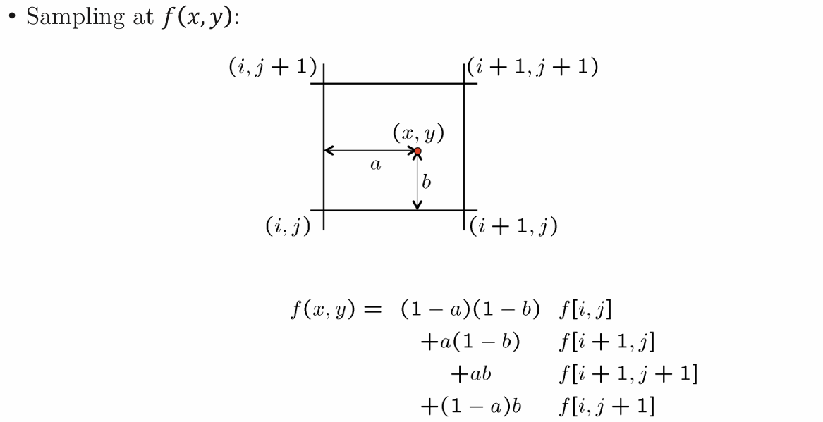
Image Stitching- Overall Procedure
• Take a sequence of images from the same position
e.g., Rotate the camera about its optical center
• Compute transformation between second image and first
Use RANSAC if necessary
• Transform the second image to overlap with the first
• Blend the two together
• If there are more images, repeat
같은 물체 다른 각도에서 찍은 사진들 가져와서 transformation 계산, 붙이기 위해 transform, blend 붙임
Week 9-2. Image Segmentation
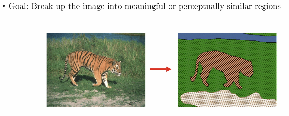
Segmentation by Humans
- Gestalt Psychology: entire먼저
- Proximity Principle: 가까운 물체는 묶음
- Similarity Principle: 비슷하면 묶음
- Common Fate: 움직임, 변화 비슷하면 묶음
- Common Region/Connectivity: 연결되면 묶음
- Continuity Principle: 연속적인 curve위에 있으면 묶음
- Symmetry Principle: 평행, 대칭 묶음
- Completion: illusory or subjective contours 환상적, 주관적 윤곽 보임
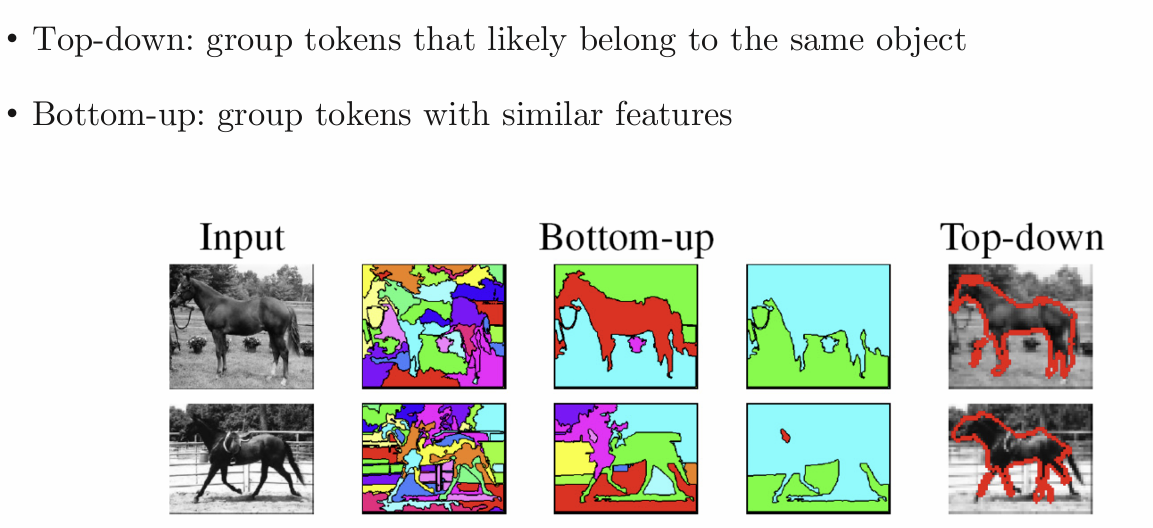
Segmentation Strategies
Top-down: 같은 물체면 묶음
Bottom-up: 비슷한 features있으면 묶음
2. K-Means Segmentation
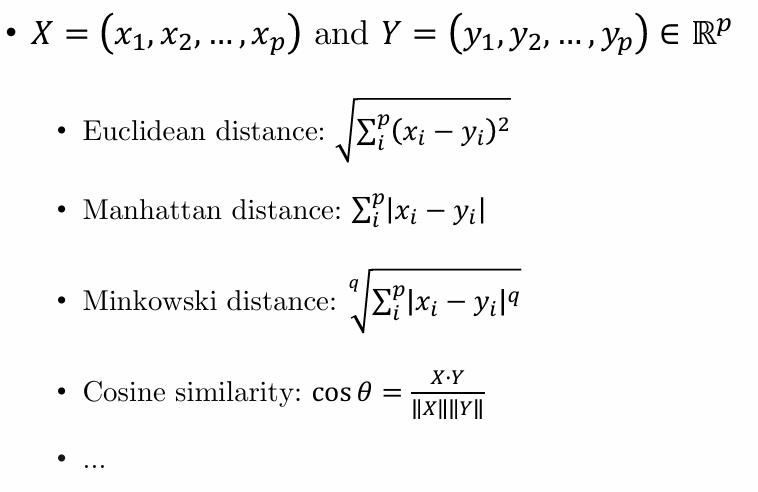
Similarity Measures
K-Means Clustering
1. Choose the number of clusters k
2. Initialize cluster centers (centroids) m1, m2,..., mk
3. For each feature point, compute the cluster center it is closest to (using some distance measure) and assign the feature point to this cluster
가장 가까운 cluster center 찾아서 cluster 정함
4. Re-compute cluster centers
5. Repeat 3 and 4 until meet the stop condition
K-Means: Initialization Methods
1. Select k random feature points as initial centroid. 너무 가까우면 resample
2. Select k uniformly distributed means within the range of the distribution 범위 안 평균
3. K-means++
Randomly pick the first centroid from the data points.
For each subsequent centroid:
Calculate the distance from each data point to the nearest chosen centroid.
Probability-weighted selection: Choose the next centroid with a probability proportional to the squared distance.
Repeat until % centroids are chosen
centroid와 거리 계산해서 제곱 거리에 비례하는 확률로 다음 중심 선택
K-Means: Stopping Criteria
1. Fixed Number of Iterations
• Stop after a predefined number of iterations.
2. Clusters Remain Unchanged
• Stop when cluster assignments no longer change between iterations.
3. Centroid Convergence
• Stop when the movement of centroids is minimal
(i.e., changes are less than a threshold, denoted as ≤ ε)
Comments
• Pros
Efficient
Easy to implement and interpret
• Cons
Requirement of cluster number
Sensitivity to initial conditions
Poor performance with non-spherical clusters 구형이 아니면 잘 못함
Sensitivity to outliers
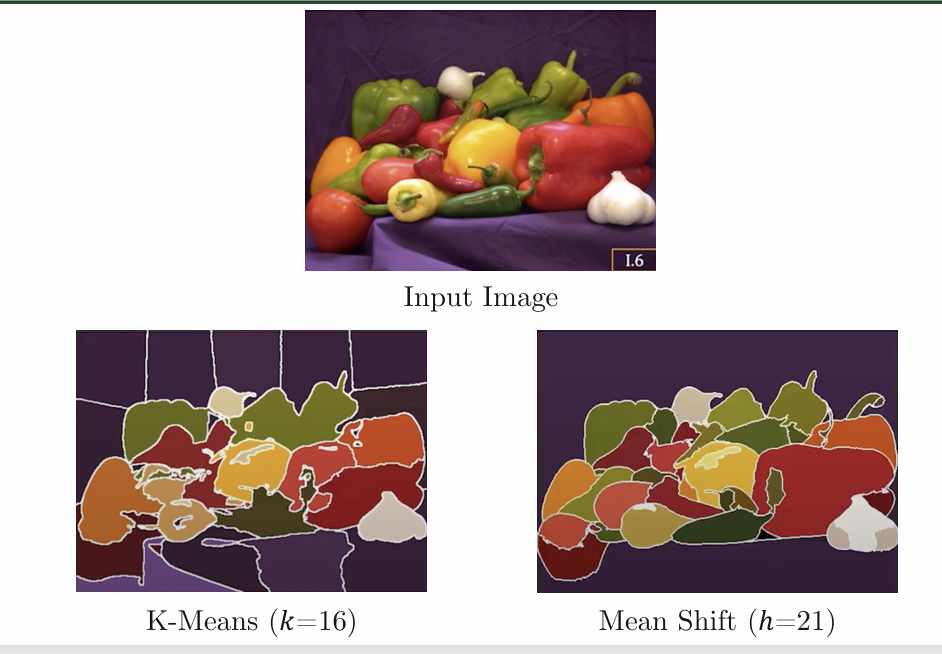
3. Mean Shift Segmentation
• Each hill represents a cluster.
• Peak (mode) of the hill represents the “center” of cluster.
• Each pixel climbs the steepest hill within its neighborhood.
• Pixel assigned to the hill (cluster) it climbs.
가장 가파른 언덕을 오름, 그 hill이 cluster
Attraction basin: the region for which all trajectories lead to the same mode 분지
Mean Shift Algorithm
The mean shift algorithm seeks modes of the given set of points
1. Choose kernel (,) and bandwidth (ℎ)
2. For each point:
a. Center a window on that point
b. Compute the mean of the data in the search window
c. Center the search window at the new mean location
d. Repeat (b, c) until convergence
3. Assign points that lead to nearby modes to the same cluster
Comments
• Pros
Simple
Finds arbitrary number of clusters
No initialization required
Robust to outliers
• Cons
Computationally expensive
Have to choose kernel size in advance
4. Graph Cut Segmentation
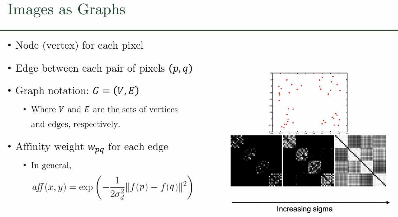
• Fully connected:
Captures all pairwise similarities
Infeasible for most images
• Neighboring pixels:
Very fast to compute
Only captures very local interactions
• Local neighborhood:
Reasonably fast, graph still very sparse
Good tradeoff
Segmentation by Graph Cuts
Break Graph into Segments
Delete links that cross between segments, low similarity
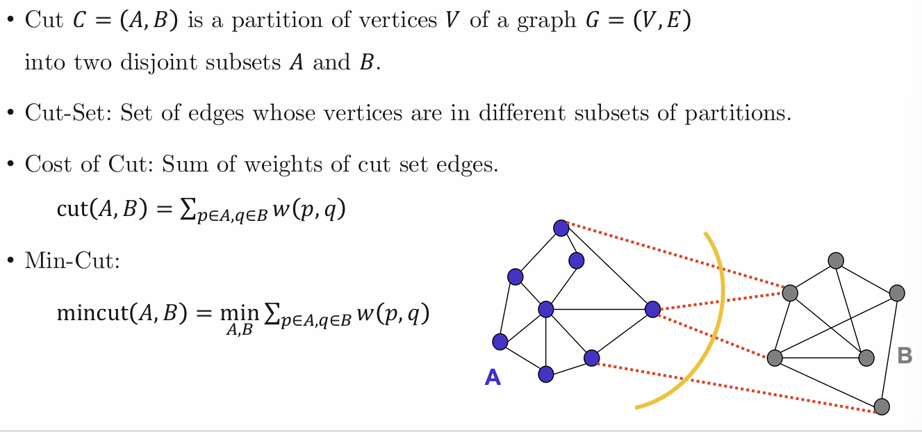
Minimum Cut
Cut-set: 끊을 edges
sum of weights가 minimum이면 cut
weight
- drawback
Weight of cut proportional to number of edges
Biased towards cutting small, isolated components
Normalized Cut
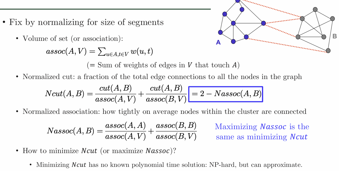
assoc(A,V)는 그래프 전체 V와 연결된 edge weight, 얼마나 큰 그래프인지
크기로 페널티, 작으면 자르기 힘듦
Nassoc는 내부적으로 얼마나 촘촘히 연결되었는지
Ncut 최소화 = Nassoc 최대화
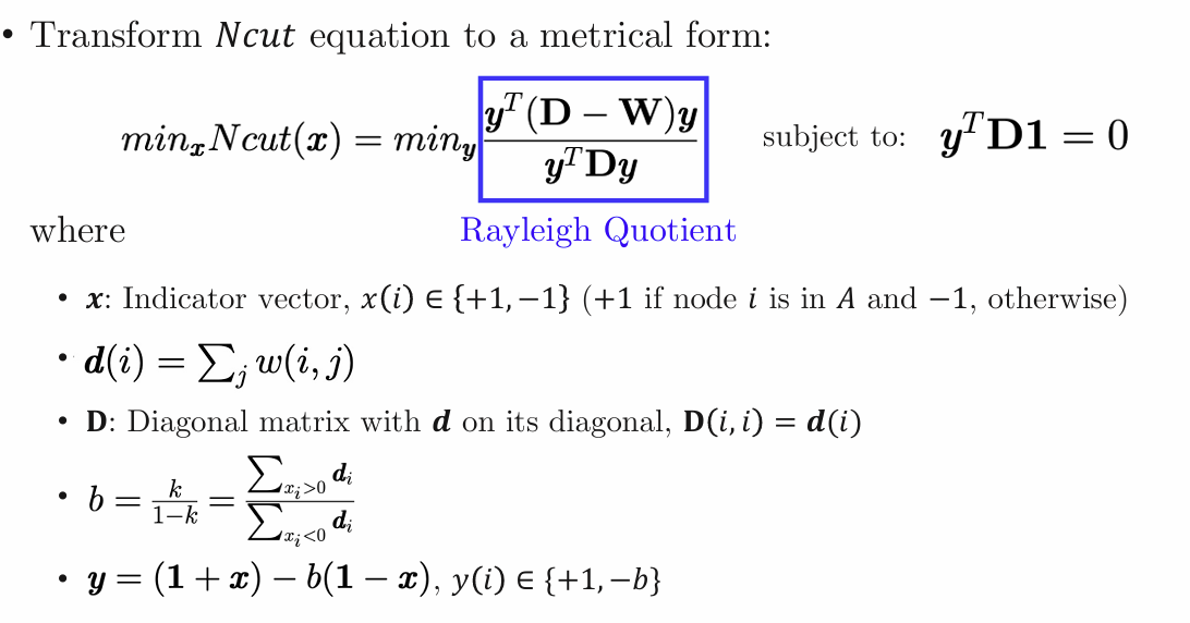
solution is given by the generalized eigenvalue problem.
optimal solution is the second smallest eigenvector
첫번째는 전체를 하나의 그룹으로 보는 것이니 두번째가 의미 있음
Comments
• Pros
Generic framework can be used with many different features and affinity formulations
Generally works better than other methods we have seen so far
• Cons
Need to choose a number of segments
High storage requirement and time complexity
Bias towards partitioning into equal segments