Lecture Week 1,2. Linear Regression with One Variable and Multiple Variables
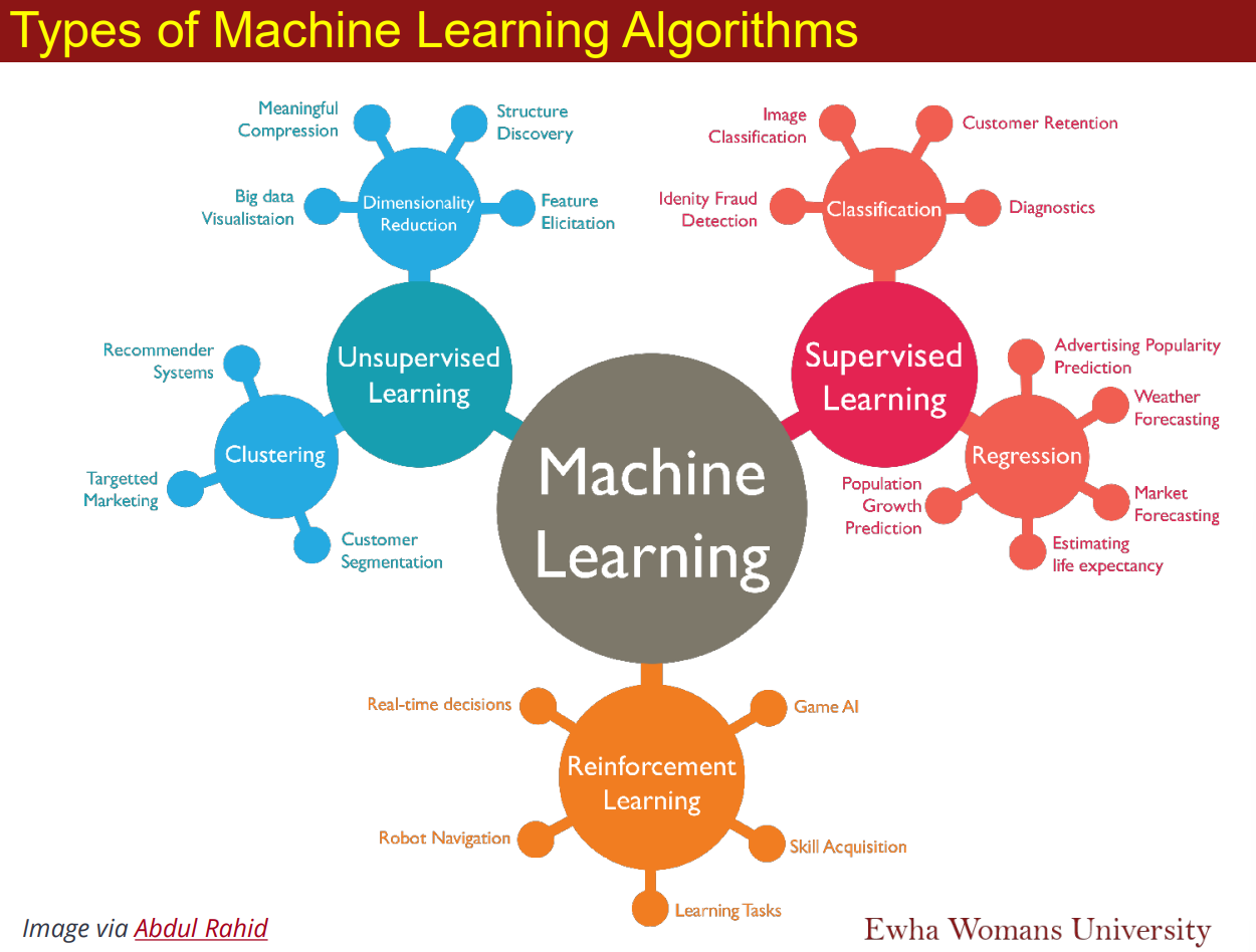
1. Supervised learning
: infers a function from labeled training data
1) Supervised Classification
Example: Spam Detection
Decide which emails are spam and which are important(not spam)
Example: Credit scoring
Differentiating between low-risk and high-risk customers from their income and savings(income, saving > a, low-risk else high-risk)
Example: Image classification, type of cancer, cancer Y/N
vs. predictions are made by classifying into different categories, discreate, categorical variable
model: Logistics Regression, Binary, Dependent variable, Decision tree, KNN, Support Vector Machines, Naive Bayes, Convolutional Neural Network
2) Supervised Regression
: Predicting numeric value
Example: Price of a used car y = wx + w0, stock market, weather prediction
vs. attempts to predict a value for an input based on past data, real number, continous numbers
model: Linear Regression, Random Forest, Multilayer Perceptron, AdaBoost, Gradient Boosting, Convolutional Neural Network
2. Unsupervised learning
: draws inferences from input data without lableled responses
1. Linear Regression with one variable
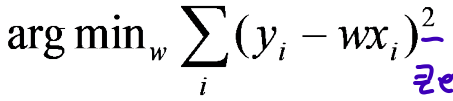
1) Numerical approach
goal: estimate w from training data of <, > pairs
optimization: minimize squared error (least squares-distance between measurements and prediction line)
estimated w, nosie:STD = 1,2..
Bias term:
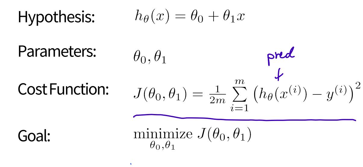
2) A cost function in Machine Learning
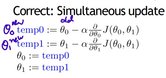
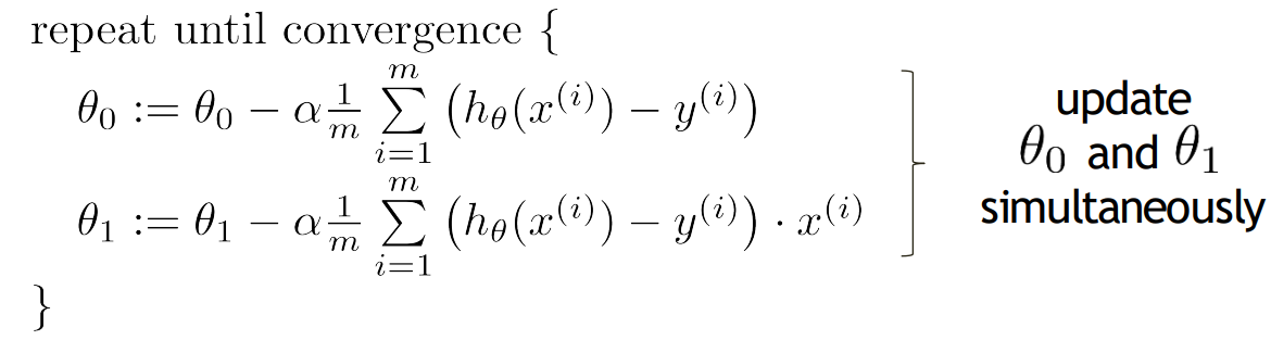
**Gradient Descent algorithm
start with some , keep changing to reduce until we hopefully end up at a minimum (simultaneously update)
repeat until convergence
(for j = 0 and j = 1)
1) Batch Gradient Descent (BGD)
: in 1 iteration, calculate gradient of all training data set and update
+Computational efficiency, stable convergence
-Convergence to local minima, Entire traing dataset must be available for each epoch
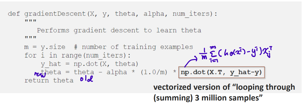
np.dot(X.T, y_hat - y) # looping 3 million samples, inefficient so SGD appear
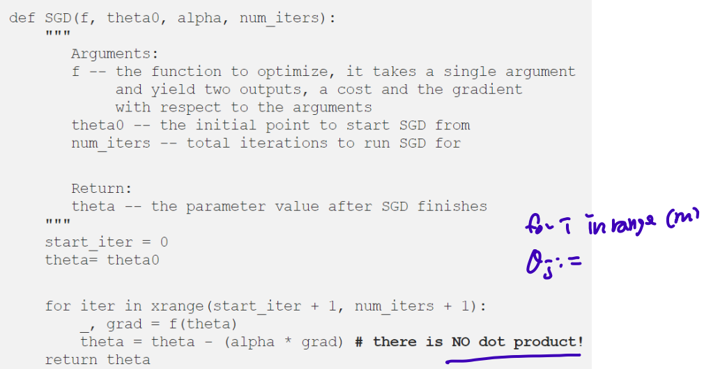
2) Stochastic Gradient Descent (SGD)
: in 1 iteration, calculate gradient of one data and update (in random data)
+Usually faster than BGD owing to sequential data processing
−Frequency of updates induces noise in gradients which affects convergence. Path to the minima is noisier.
−Frequent updates are computationally expensive
+) Mini Batch Gradient Descent (MGD)
: in 1 iteration, calculate average gradient of train data in one mini batch and update
uses n data points (instead of 1 sample in SGD) at each iteration.
Intuition1: which way to go
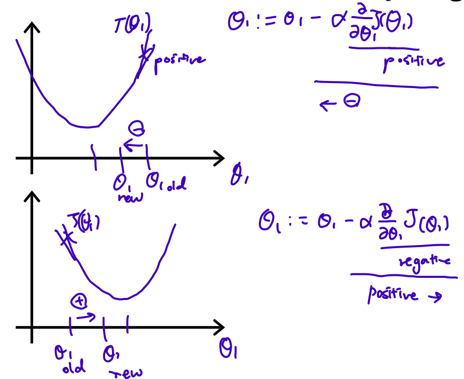
positive decrease, move left
negative increase, move right
Intuition2: learning rate
learning rate step size
When the learning rate is too low, it takes a lot of steps to converge
When the learning rate is too high, Gradient Descent fails to reach the minimum
Gradient descent for linear regression
- recap quiz(pseudo code)
%% cost function
[theta,theta1] = meshgrid(-1000:1:1000);
for i = 1:2001
	for j = 1:2001
		sum=0;
		for k=1:length(x)
			sum = sum + [theta(i,j) + theta1(i,j) * x(k) - y(k)]^2;
		end
		Z(i,j) = sum/(2*length(x));
	end
end
figure(1) ;
mesh(theta,theta1,Z);
[r c]=min(Z);
title('Graph of Cost Function vs Parameters');
xlabel('\theta_0');
ylabel('\theta_1');
zlabel('Cost Funtion')

%% gradient descent for linear regression
alpha=.01;
psi=0;
psi1=0;
for i=1:5000
	sum1=0;
	sum2=0;
	for j=1:length(x)
		sum1=sum1+(psi+psi1*x(j)-y(j));
		sum2=sum2+(psi+psi1*x(j)-y(j))*x(j);
	end
	psi=psi-alpha*sum1/length(x);
	psi1=psi1-alpha*sum2/length(x);
End

fprintf('The theta0 value is = %d', psi);
fprintf('\n\nThe theta1 value is = %d\n\n', psi1);
for i=1:length(x)
	xnew(i)=x(i);
	ynew(i)=psi+psi1*x(i);
end
figure(2); scatter(x,y,'x','r'); hold on;
title('Graph of DATA vs PREDICTED FIT');
plot(x,ynew,'g');hold off;
legend('DATA','PREDICTED FIT');
xlabel('x'); ylabel('F(x)')
%% theta0 = 1.2, theta1 = 0.4
2. Linear Regresssion with Multiple Variables
: Learning/ optimizing multivariate least squares using gradient descent
(variable x)
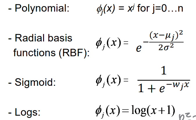
Non-Linear basis function
: add an intercept term(절편함), add a new variable z = 1 and weight (data 원하는 형식에 맞게 범위나 모양을 바꿈)
general notation:
for multivariate regression or non-linear basis function
=1 for the intercept term
Gradient Descent for Multivariate Linear Regression
Goal: minimize loss function(g)
- Learning algorithm:
initialize weights w=0
for t=1, until convergence:
Predict for each example using w: # find
Compute gradient of loss
Update: (: learning rate)
+)
(i: sum n examples, j: sum k+1 basis vectors)
Regression and Overfitting/ Underfitting
- Bias-Variance Tradeoff
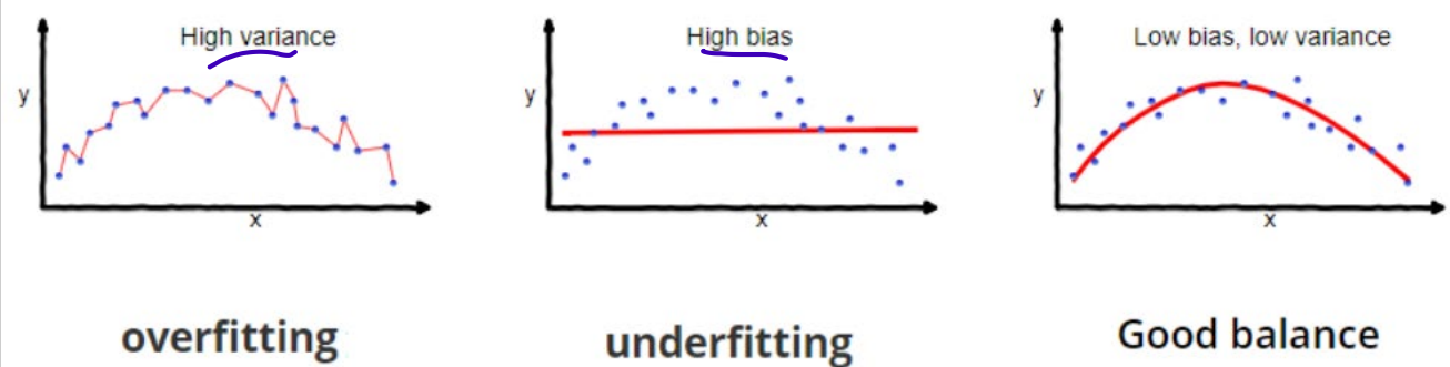
Overfitting: high variance
too many hypotheses, expressive class
error on the training data is very low, but error on new instances is high
Underfitting: high bias
not having good hypotheses, less expressive class
- How to overcome overfitting issue?
Train with more data
Remove features (regularization): add sum of weights to loss function so that push some weights towards zero
Early stopping (validation)
Ensembling (bagging, boosting)
Regularization
: add information to prevent overfitting
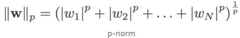
- L1 regularization (lasso regression)
: add sum of weights to loss function so that some weights become zero.
sum of weights, less sensitive to outlier, penalize small values more; feature selection, effect on pushing towards 0 (sparsity) - L2 regularization (ridge regression)
: add squared weights to loss function so that some weights become close to zero.
squared weights, penalizes large values more
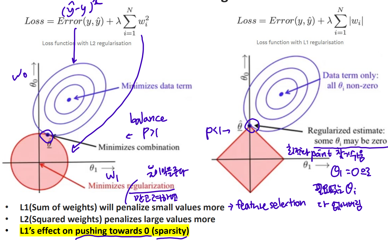
은 feature weight, 타원 그래프의 중심에 가까워질수록 데이터는 최적화한다. minimize data term
타원 그래프의 중심에 가장 가까우면서 정규화 그래프(규제영역)와 만나는 부분이 minimize combination. 이는 한 feature를 없앨 수도 있다. ()
Cross-validation
: generate multiple mini train-test splits and use these splits to tune your model (ith validation set, k-1 training set, test set for i=1tok)
- general procedure for estimating the true error of a predictor:
use a training and validation set to find the right predictor
use a test set to report the prediction error of the algorithm
repeated several times, results are averaged
Leave-one-out cross-validation
(one instance)
1. for each order of polynomial d:
- repeate m times:
1) leave out ith instance from the training set and put in a validation set
2) find best parameter vector using other instances
3) measure the error using ith instance, (unbiased estimate of the true prediction error - Compute the average of the estimated errors
- Choose the d with lowest average estimated error:
+) order of polynomial d, parameter: d=d일때 validation set을 m번 뽑아 즉 erorr를 m번 구하고 이를 평균내서 즉 avgerage of estimated error구함. 구한 중 최솟값을 가지는 d를 구함
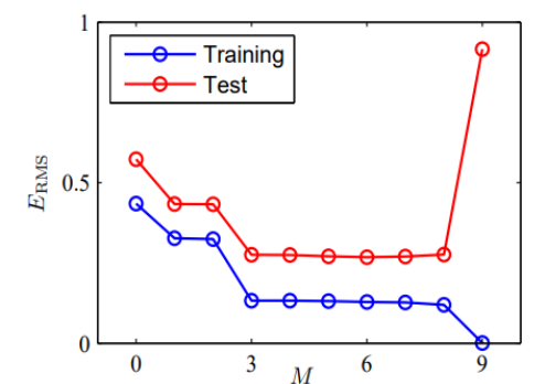
As d increases, the training error decereases
but the validation error decreases, then starts increasing again
d right before the increase is optimal
- summary:
computational cost scales with the number of instances, so prohibitive if finding the best predictor is expensive
+) k-fold cross-validation: split the data set into k parts, then proceed as above