[ML] 3. Neural Networks

Week 4-1. Neural Networks

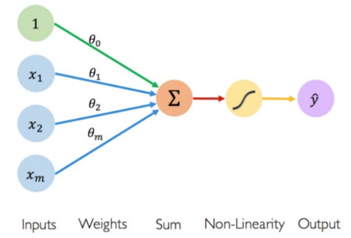
• Neuron unit

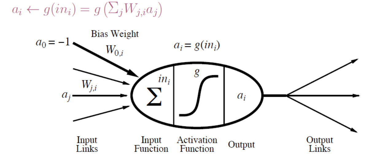
• activation functions

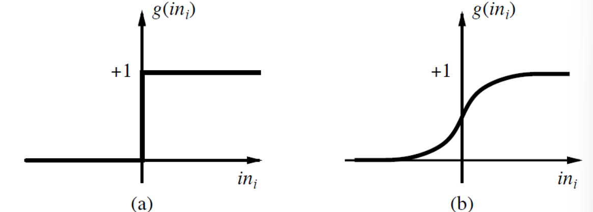
(a) step/threshold function, (b) sigmoid function $\frac{1}{1 + e^{-x}}$
Changing the bias weight $W_{0,i}$ moves the threshold location

Network structures: Feed-forward networks

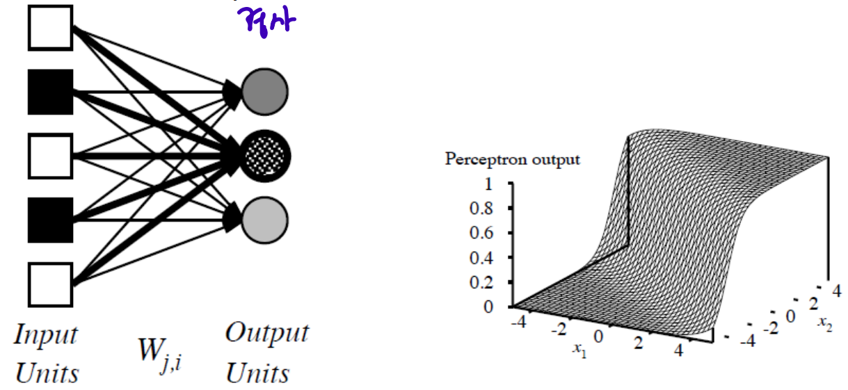
1. Single-layer Perceptrons

use a step/sigmoid function as activation function
output units all operate separately-no shared weights
adjusting weights changes the cliff's location, orientation, and steepness(경사)

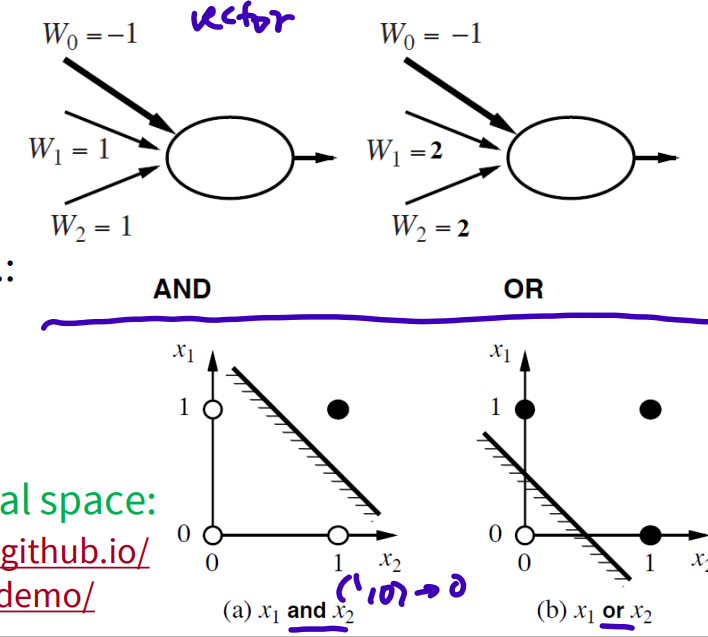
• Perceptron learning: Linearly-Separable Functions

can represent AND, OR, NOT, majority, etc.. but not XOR (2-dimensional space)
$\sum_jW_jx_j > 0$ -> 1
$\sum_jW_jx_j \leq 0$ -> 0
$x_j$ = 0 or 1

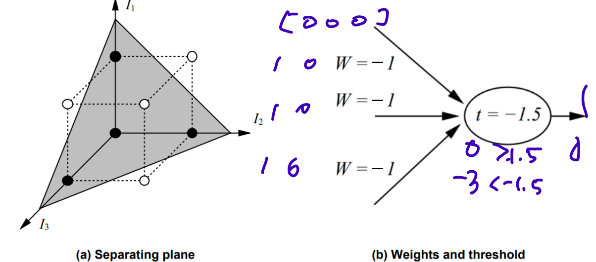
3-dimensional space: the minority function- return 1 if 1s < 0s; return 0 otherwise

2. Multi-layer Perceptrons

the number of layers: counted except the input layer

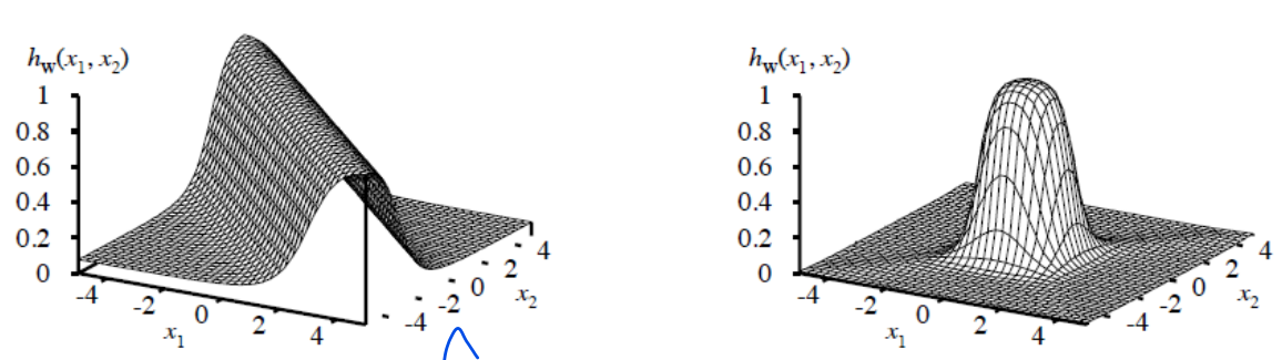
combine threshold functions-ridge-bump (능선/봉우리-혹)

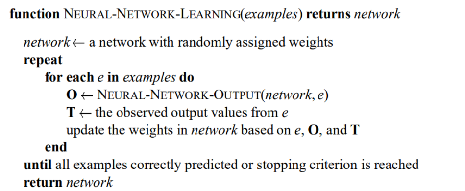
• Learning with NNs
  

Recurrent networks
directed cycles with delays, internal state

Week4-2 Neural Networks: Activation function, Building networks

Activation functions

must be non linear, differencialable/ better zero centered(bounded)
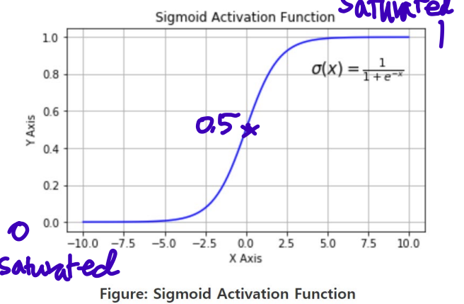
1. Sigmoid
drawbacks: Vanishing gradient, not zero centered, computationally expensive

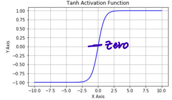
2. Tanh
   Zero-centered & squashed
   Vanishing gradient

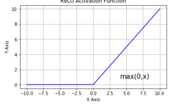
3. ReLU (Rectified Linear Unit)
   Not zero-centered, vanishing gradient when x < 0

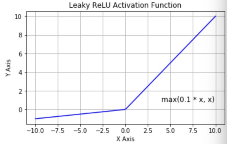
4. Leaky ReLU

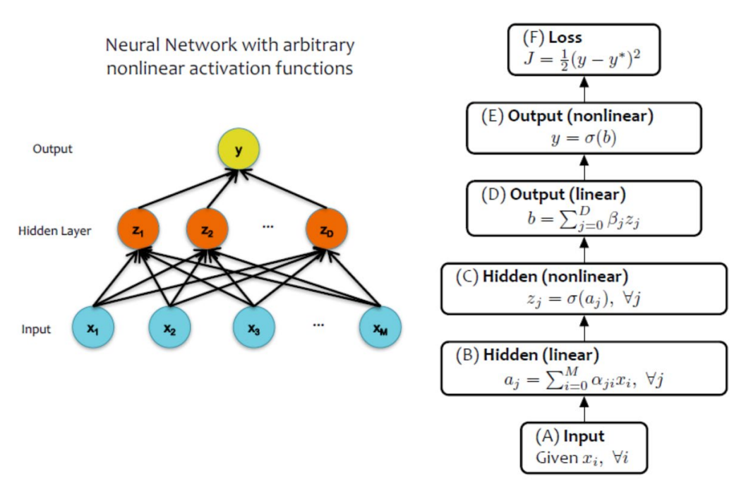
Building a Neural Net

1. # of hidden layers (depth)
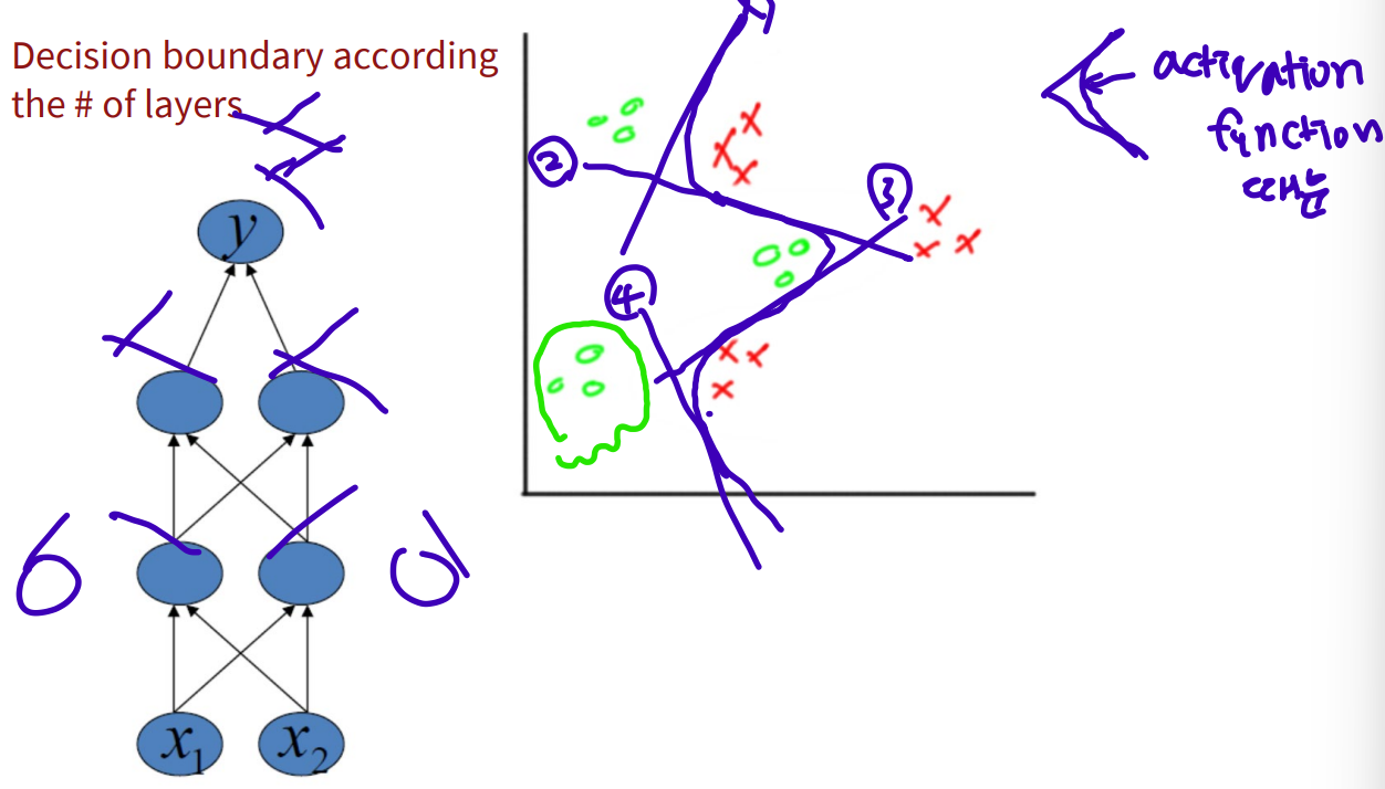
Decision boundary according to the number of layers
1 hidden layer: boundary of convex region
2 hidden layer: combinations of convex region

2. # of units per hidden layer (width)
size of hidden layer D, size of input M
D = M
D < M: encoded, feature extraction, classification
D > M: optimal, diverse features, can be overfitting

3. Types of activation function (nonlinearity)

4. Form of objective function
Regression: same objective as Linear Regression, quadratic loss (mean squared error)
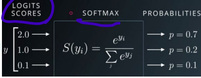
Classification: same objective as Logistic Regression, cross-entropy (negative loglikelihood), softmax layer

Lecture Week 5-1. Neural Networks: Back-propagation

Recall gradient descent algorithm

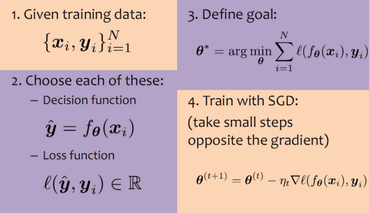
Forward- & Back-propagation

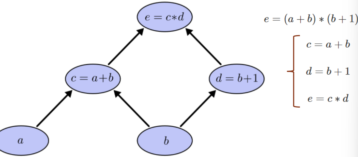
• Computational graph
  nodes correspond to operations or variables

• Functions as boxes

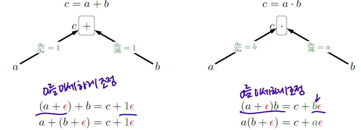
(a + $\epsilon$) -> c + gradient*$\epsilon$

Linear classification with hinge loss (linear problem)

• find loss function and its gradients (setting)

$Loss(x,y,w) = \max\{1 - w\cdot\phi(x)y, 0\}\\ \nabla_w Loss(x,y,w) = -\phi(x)y$ (margin < 1)
margin = $w\cdot\phi(x)y$ if margin >= 1, 0

Two-layer neural networks

$h(x) = V\phi(x)\\ f_{V,w}(x) = sign(w\cdot h(x))$
$Loss(x,y,V,w) = (w\cdot\sigma(V\phi(x)) - y)^2 = (\hat{y} - y)^2 = (residual)^2\\ \nabla_w Loss(x,y,V,w) = 2(residual)h\\ \nabla_V Loss(x,y,V,w) = 2(residual)w\cdot h\cdot (1-h)\phi(x)^T$

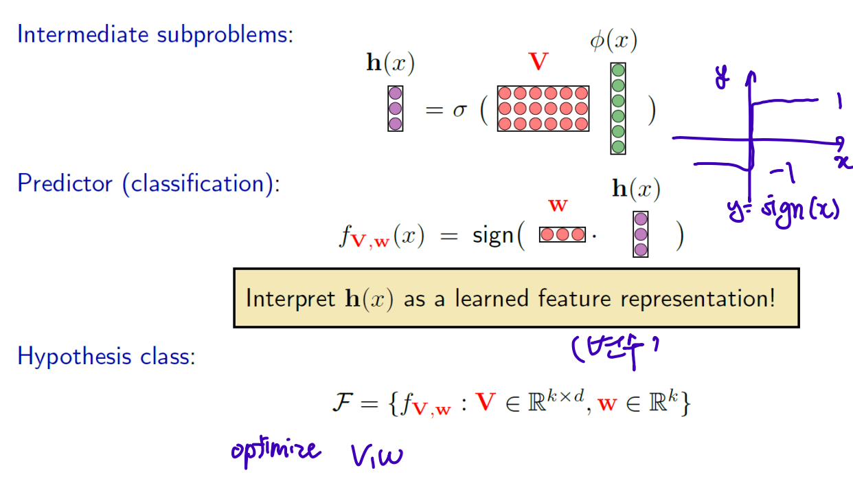
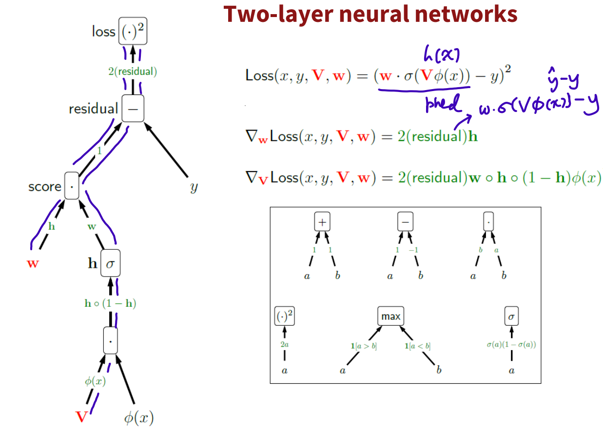
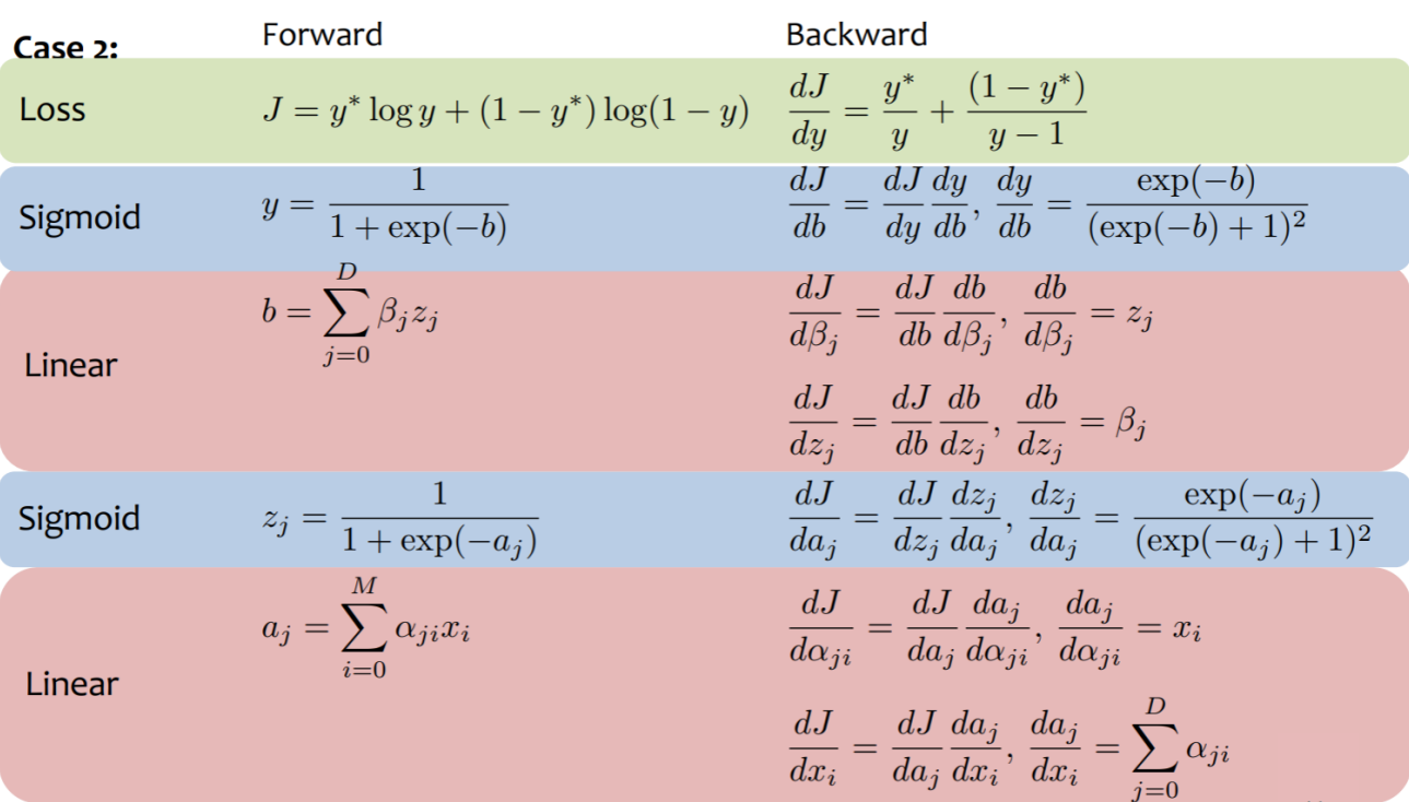
Backpropagation

1. Backpropagation for Logistic regression model or 1-layered Neural Network Model

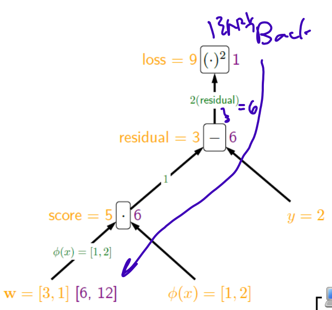
orange: forward calculation
purple: back 1 -> 1 * 2(residual) = 6 -> 6 * 1 = 6 -> 6 * [1,2] = [6,12]
old * gradient

• Derive the formula for gradient descent algorithm

Cost Function $J = -yloga - (1 - y)log(1 - a)\\ z = w_1 x_1 + w_2 x_2 + b$
$\hat{y} = h_\theta(x) = \sigma(z) = a$ -> $J = L(a,y)$

$\displaystyle \frac{\partial L}{\partial w_1} = \frac{\partial L}{\partial a}\cdot\frac{\partial a}{\partial z}\cdot\frac{\partial z}{\partial w_1}$

$\displaystyle \frac{\partial L}{\partial a} = \frac{-y}{a} + \frac{1-y}{1-a},\;\displaystyle \frac{\partial a}{\partial z} = a(1 - a),\; \frac{\partial z}{\partial w_1} = x_1$

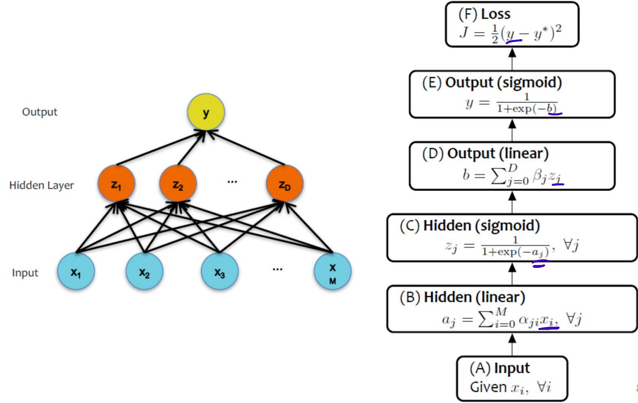
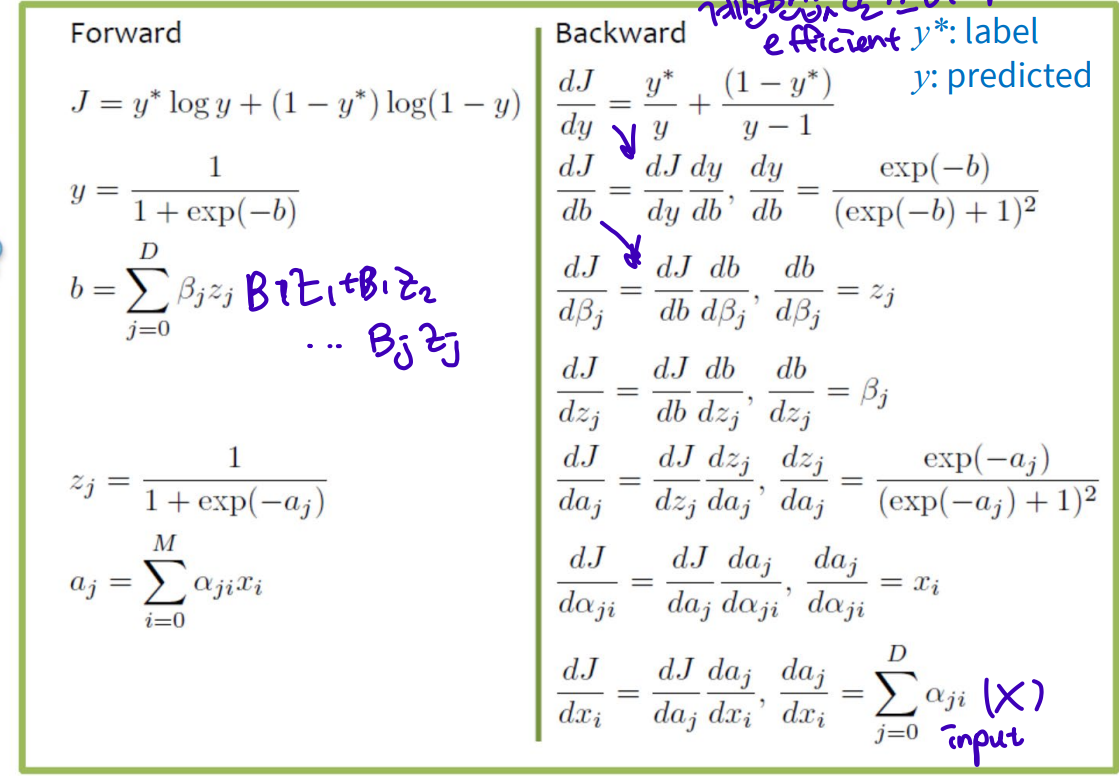
2. Backpropagation for 2-layered Neural Network

Lecture Week 7-1. Neural Network: Practice building Neural Networks w/MNIST

MNIST number classification

:Mixed National Institute of Standards and Technology database
0-9 handwritten digit recognition
train:test = 6:1
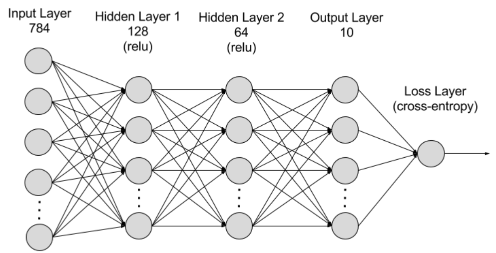
Multilayer Perceptron network architecture for MNIST for today's practice

Data Normalization/ Feature Scaling: Data Preprocessing

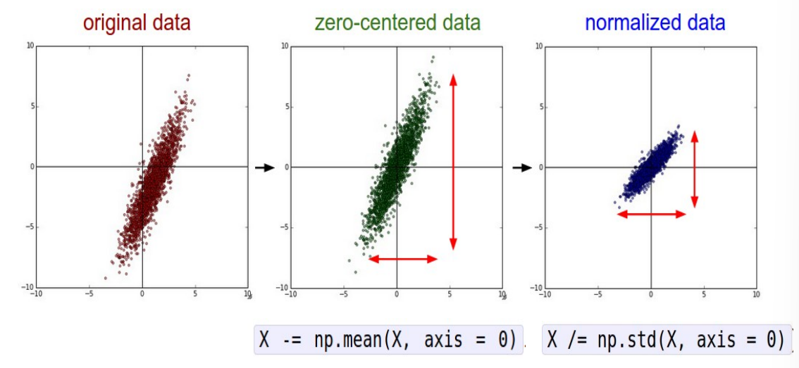
Advantages: classification loss becomes less sensitive to small changes in weights; easier to optimize

Mini-batch SGD

after creating the mini-baches of fixed size, in one epoch:
1. Pick a mini-batch (100)
2. Feed it to Neural Network
3. Calculate the mean gradient of the mini-batch
4. update the weights using the mean gradient
5. Repeat steps 1-4 for the mini-batches

: balance between the robustness of SGD and the efficiency of BGD
smaller batch size -> more updates, more time, lower speed
very large batch size can yield wore performance

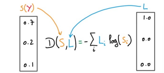
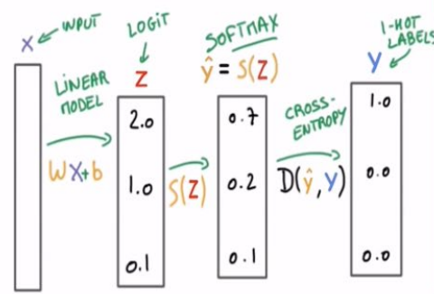
Cross-entropy loss for classification

• Binary cross-entropy loss
  $\displaystyle H_{y'}(y) := -\sum_i(y'_i log(y_i) + (1 - y'_i)log(1 - y_i))\\ y_i$: predicted probability for class i, $y'_i$: true probability for class i

• Cross-entropy loss for multi-class classification
  $\displaystyle H_{y'}(y) := -\sum_i y'_i log(y_i)$
  If target = 1, the loss is 0 when the prediction is 1 and loss is infinity when the prediction is 0

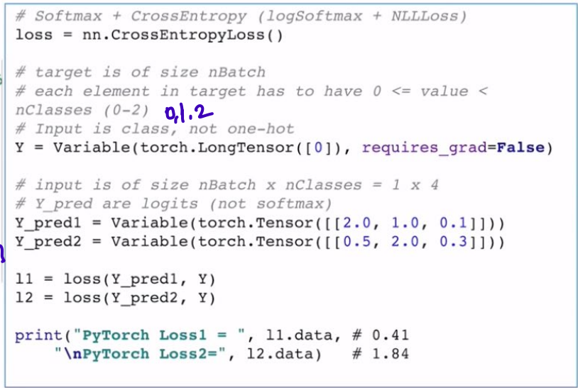
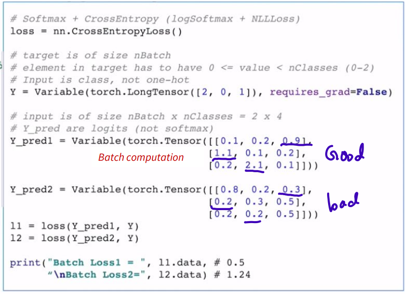
• Cross-entropy in PyTorch
  combine nn.LogSoftmax() and nn.NLLLoss()
  recall softmax: $\displaystyle \sigma(z)_j = \frac{exp(z_j)}{\sum^K_{k=1}exp(z_k)}$ for j = 1, ..., K.
  recall cross-entropy: $D(\hat{Y}, Y) = -Ylog\hat{Y}\\ \hat{Y} = S(Z)$

??

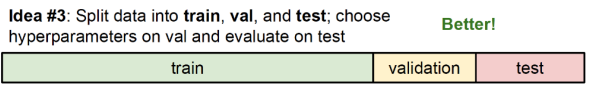
Traning, Validation, Test Set

• Train data
• Validation data: use training error and validation error to determine when to stop to prevent overfitting (early stopping)
• Test data: measure the generalization ablility of a machine learning algorithm. never seen during the training process