한번 정리했던 내용이지만, 한번 더 해보면서 기억을 다져보자..!

1. Introduction

Vision task에서 CNN은 backbone으로 널리 사용되고 있고, NLP task에서는 transformer가 long range dependencies 문제 해결과 관련해 널리 사용되고 있음.

• Transformer + Image domain= Vision transformer

Language domain에서의 high performance를 image domain으로 옮겨올 때 가장 큰 challenge?

→ Domain 간 modality의 차이!

1. NLP에서는 각 단어가 basic token의 역할을 하지만 vision에서는 basic token이 scale에 따라 변할 수 있음

   : 반대로, vision에서 transformer 기반 모델들의 token이 고정된 scale을 가지면 변화하는 scale에 유연하게 적용할 수 없어 적합하지 않음

1. NLP에서 한 문장 또는 문단의 단어 수보다 이미지의 pixel 수가 훨씬 많음(higher resolution)

   : 높은 해상도의 pixel 단위 task(Segmentation, Depth Estimation…)에 대해 NLP의 임베딩 방식을 그대로 가져오면 해상도 차이 때문에 token이 pixel 단위만큼 이미지를 잘 표현할 수 없음

   💡 Swin Transformer(Shifted Window Transformer)*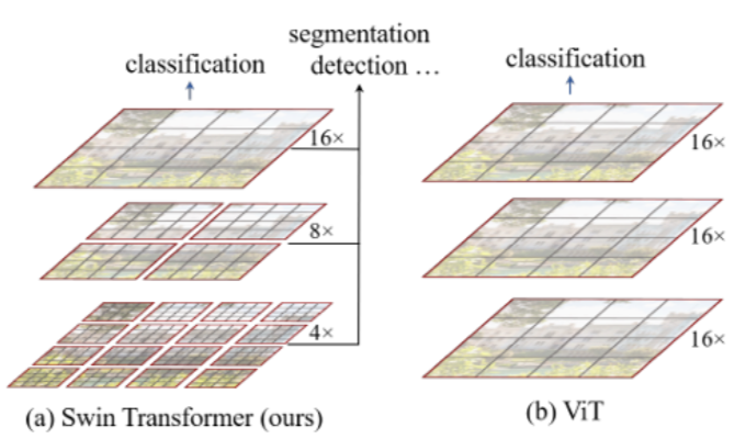

   

https://openaccess.thecvf.com/content/ICCV2021/papers/Liu_Swin_Transformer_Hierarchical_Vision_Transformer_Using_Shifted_Windows_ICCV_2021_paper.pdf

• 작은 size의 patch에서 계속 merge 해가며 점점 큰 attention map 생성 : 작은 크기의 패치를 하나의 단위(basic token)로 삼고 패치를 합쳐가며 크기를 늘려가는 방식
  • Image 크기에 대해 computational complexity가 linear하게 증가
  • 연속된 transformer layer 사이 window가 움직이는 방식(shifted window)으로 동작

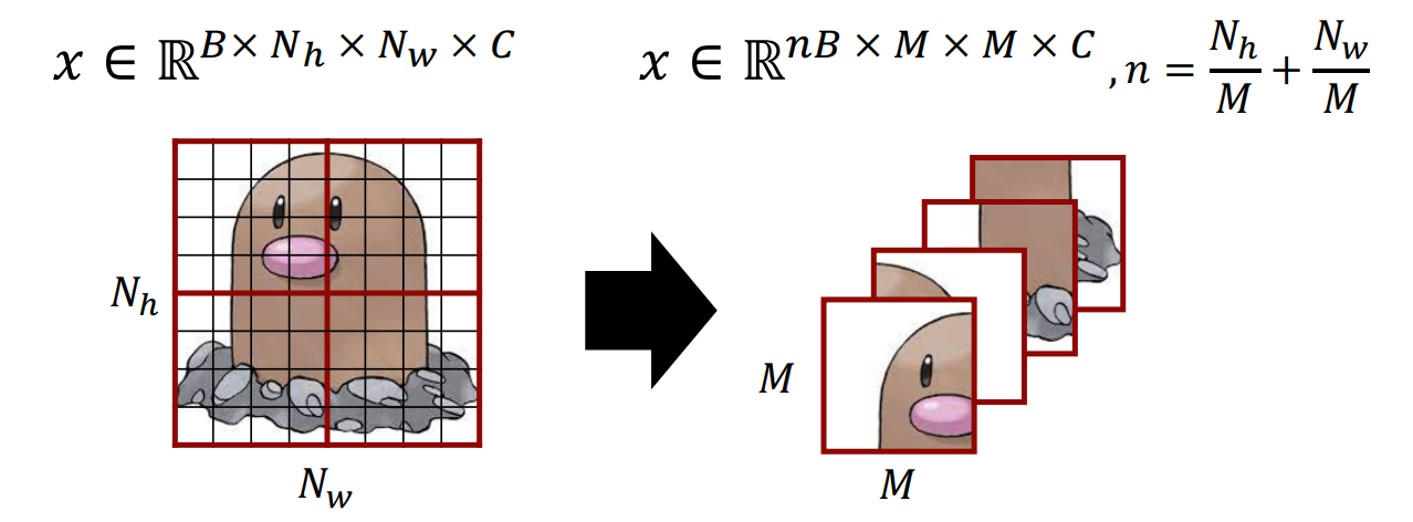
Patch size: $\small 4\times 4$

2. Related Works

CNN

• Alexnet부터 주목을 받기 시작한 CNN은 비전 전반에서 backbone으로 많은 역할을 함
• 이후 ResNet, DenseNet, Mobilenet 등 CNN 기반 네트워크들이 등장하면서 depthwise convolution 등 다양한 기법 제안

Self-attention based backbone architectures

• Resnet의 일부 layer을 self-attention으로 대체하려는 시도
• local pixel에 대한 sliding window 방식의 경우 메모리 문제로 latency가 매우 컸음

Self-attention/Transformers to complement CNNs

• Self attention 구조를 통해 CNN 기반 네트워크의 구조를 늘리려는 시도
• Encoder(backbone), head network 등에 사용. 본 논문에서는 feature extractor로 사용

Transformer based vision backbones

• 기존의 ViT는 resolution이 높은 이미지나 dense prediction task에 대해서 general한 backbone이 되기 어려움 (token issue!)
• ViT를 dense vision task에 적용하거나 ViT의 구조 자체를 변경하려는 시도

3. Methods

3.1. Overall Architecture

https://openaccess.thecvf.com/content/ICCV2021/papers/Liu_Swin_Transformer_Hierarchical_Vision_Transformer_Using_Shifted_Windows_ICCV_2021_paper.pdf

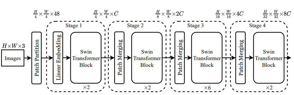
1. Stage 1

• $\small P^2C=4^2\times3=48$ : Embedding 전 single patch vector 크기
• $\small N_p={HW\over 16}$ : Window 안 patch(이하 token) 개수

→ $\small ({H\over 4} \times {W\over 4})\times 48$

• Linear embedding: 임의의 feature dimension(이하 C) 로 임베딩

  → $\small ({H\over 4} \times {W\over 4})\times C$

• Swin transformer block을 두 번 거쳐 $\small ({H\over 4} \times {W\over 4})\times C$ 크기의 matrix 출력

2. Stage 2

• Patch merging layer: 이웃한 2x2 token들을 concat:

: $\small ({H \over 8}\times {W\over 8})\times 4C$

• Token 내부 vector 크기를 4C에서 2C로 project (Fully connected)

: $\small ({H \over 8}\times {W\over 8})\times 2C$

• Swin transformer block을 두 번 거쳐 $\small ({H \over 8}\times {W\over 8})\times 2C$ 크기의 matrix 출력

3. Stage 3

• Patch merging layer: 이웃한 2x2 token들을 concat: : $\small ({H \over 16}\times {W\over 16})\times 8C$
  
• Token 내부 vector 크기를 8C에서 4C로 project (Fully connected) : $\small ({H \over 16}\times {W\over 16})\times 4C$
  
• Swin transformer block을 여섯 번 거쳐 $\small ({H \over 16}\times {W\over 16})\times 4C$ 크기의 matrix 출력

4. Stage 4

• Patch merging layer: 이웃한 2x2 token들을 concat: : $\small ({H \over 32}\times {W\over 32})\times 16C$
  
• Token 내부 vector 크기를 16C에서 8C로 project (Fully connected) : $\small ({H \over 32}\times {W\over 32})\times 8C$
  
• Swin transformer block을 두 번 거쳐 $\small ({H \over 32}\times {W\over 32})\times 8C$ 크기의 matrix 출력

5. Swin Transformer block

https://openaccess.thecvf.com/content/ICCV2021/papers/Liu_Swin_Transformer_Hierarchical_Vision_Transformer_Using_Shifted_Windows_ICCV_2021_paper.pdf

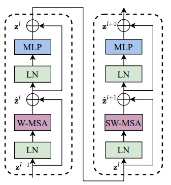
• Swin transformer block 은 두 개의 ViT block이 연결된 형태
• MLP의 activation으로는 GELU를 사용
• W-MSA는 기존 multi-head self attention 모듈을, SW-MSA는 shifted multi-head self attention 모듈을 의미

3.2. Shifted Window based Self-Attention

• Standard transformer에서 사용한 attention 연산은 global attention이기 때문에 토큰의 개수(이미지 크기)에 따른 quadratic computation complexity를 가짐
• Token의 개수를 많이 필요로 하는 vision task(Dense prediction, High resolution image) 등에 부적합 할 수 있음

Self attention in non-overlapped windows

Class token이 있을 때를 가정하며, MSA는 SA를 나눠서 수행한 것이므로 computational complexity가 동일하기 때문에 아래는 SA로 계산

노란색 표시가 연산량!

• $\small P$ : Image patch의 한 변의 픽셀 수
• $\small N_p={HW\over p^2}$ : # patches
• $\small D$ : embedding dimension
• $\small x_p$ : matrix of flattened patches → $\small (N_p+1,\ P^2C)$
• $\small w$ : weight. self attention → $\small (D,\ D)$

일반적인 vision transformer

1. $\small z=x_p \cdot E$ : embedding → $\small (N_p+1)\times D$ : $\small D\times (N_p+1)\times P^2C$

2. $\small q=z\cdot w_q$ : $\small D^2(N_p+1)$

3. $\small k=z \cdot w_k$ : $\small D^2(N_p+1)$

4. $\small v=z\cdot w_v$ : $\small D^2(N_p+1)$

5. $\small A={qk^T \over \sqrt D}$ : $\small (N_p+1)^2D$

6. $\small SA=A\cdot v$ : $\small (N_p+1)^2D$

7. (Weighted)$\small SA=SA\cdot w_z$ : $\small D^2(N_p+1)$

   P가 고정일 때 $\small N_p$는 $\small HW$에 dependent하므로 $\small N_p+1\approx N_p=HW\times k$ ($\small k$: constant)

   P가 고정이 아니면 P가 증가함에 따라 embedding 과정에서의 complexity가 quadratic하게 증가함!

원문 github에서도 Patchembed 함수에서 patch size를 argument로 받는것을 확인할 수 있음

Swin-Transformer/swin_transformer.py at main · microsoft/Swin-Transformer

$\small \Omega (SA)= kDP^2C(HW)+4kD^2(HW)+ 2k^2D(HW)^2$

→ $\small HW$ 에 대해 $\small O(N^2)$ : Quadratic

Swin transformer

전체 이미지를 $\small M\ \times \ M$ 크기의 window로 나누었다고 가정할 때 patch 수 $\small N_p+1$ 은 $\small HW$가 아닌 $\small M^2$에 비례하지만 윈도우 개수가 $\small {H\over M}\times {W\over M}$ 개로 늘어남.

1. $\small z=x_p \cdot E$ : embedding → $\small (N_p+1)\times D \times {HW\over M}$ : $\small D\times (N_p+1)\times P^2C\times {HW\over M^2}$
2. $\small q=z\cdot w_q$ : $\small D^2(N_p+1)\times {HW \over M^2}$
3. $\small k=z \cdot w_k$ : $\small D^2(N_p+1)\times {HW \over M^2}$
4. $\small v=z\cdot w_v$ : $\small D^2(N_p+1)\times {HW \over M^2}$
5. $\small A={qk^T \over \sqrt D}$ : $\small (N_p+1)^2D\times {HW\over M^2}$
6. $\small SA=A\cdot v$ : $\small (N_p+1)^2D\times {HW\over M^2}$
7. (Weighted)$\small SA=SA\cdot w_z$ : $\small D^2(N_p+1)\times {HW\over M^2}$

$\small N_p+1\approx N_p= M^2\times k$ ($\small k$: constant)

$\small \Omega (W-SA)= kDP^2C(HW)+4kD^2(HW)+2k^2M^2D(HW)$

→ $\small HW$에 대해 $\small O(N)$: Linear

논문에서는 Embedding 과정을 생략하고 아래와 같이 표기

$\small \Omega(MSA)=4hwC^2+2(hw)^2C$

$\small \Omega(MSA)=4hwC^2+2M^2hwC$

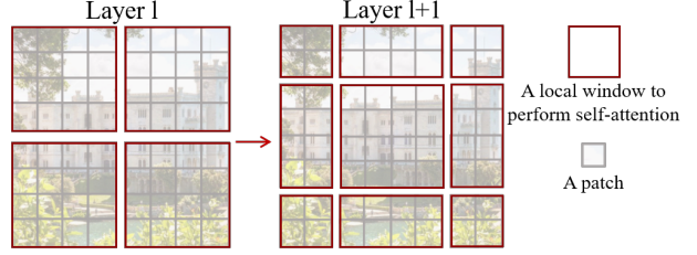
Shifted window partitioning in successive blocks

• Window based attention model은 window간 정보를 서로 반영하기 어렵다는 단점이 있음
• Cross window connection을 적용하면서 non-overlapping window의 장점을 보존할 수 있는 방법
  

(https://openaccess.thecvf.com/content/ICCV2021/papers/Liu_Swin_Transformer_Hierarchical_Vision_Transformer_Using_Shifted_Windows_ICCV_2021_paper.pdf)](https://s3-us-west-2.amazonaws.com/secure.notion-static.com/3d4dc3d7-3474-4910-886d-996e69a947ab/Untitled.pn

• Layer1에서는 일반적인 window partitioning 후 Window Multi Head Attention을 수행하고 Layer 2에서 Shifted Window Multi Head Attention(SW-MSA) 수행 [(위의 그림 참고)]

https://openaccess.thecvf.com/content/ICCV2021/papers/Liu_Swin_Transformer_Hierarchical_Vision_Transformer_Using_Shifted_Windows_ICCV_2021_paper.pdf

Efficient batch computation for shifted configuration

• Efficient batch computation

$\ \ \ \ \ \ \ \ \ \ \ \ \ \ \ \ \ \ \large x \in \R^{ 1\times 16\times 16\times 3}$ $\large\ \ \ \ \ \ \ \ \ \ \ \ \ \ \ \ \ \ \ \ \ x\in\R^{\red 4\times 8\times 8\times 3}$

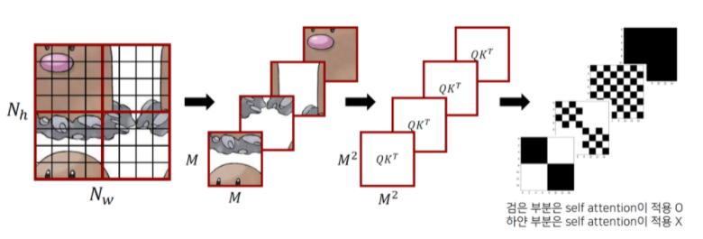
각 Window에 대해 4번 연산할 내용을 batch 단위로 끌어와서 연산 효율성 증가!

• SW-MSA
  • Window를 $(\llcorner {\small M\over2}\lrcorner, \llcorner {\small M\over2}\lrcorner)$ 픽셀만큼 좌측 상단으로 이동 → Cyclic shift

https://openaccess.thecvf.com/content/ICCV2021/papers/Liu_Swin_Transformer_Hierarchical_Vision_Transformer_Using_Shifted_Windows_ICCV_2021_paper.pdf

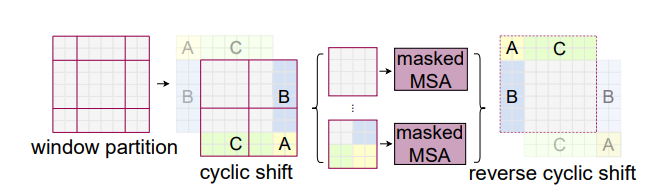
• A, B, C 는 좌상단 큰 부분과 기존 인접한 부분이 아니기 때문에, 좌상단 부분만 masking을 거쳐 self-attention 적용
  • Attention$\small (Q,K,V)$=Softmax$\small (QK^T/\sqrt d+B)$$\small V$ → $\small QK^T$는 $\small M^2\times M^2\ \ (N_p+1\times N_p+1)$
  • Mask 모양도 $\small M^2 \times M^2$가 되어야함
    
    

출처: http://dsba.korea.ac.kr/seminar/?mod=document&pageid=1&keyword=swin transformer&uid=1793, 고려대학교 DSBA 연구실 Swin Transformer 발표자료

• 위의 그림에서 마지막이 attention mask, 검정색 부분이 0, 하얀색 부분이 -100
  • Mask가 더해지는 형태이므로, -100이 더해지면 activation이 0에 가까워져 attention이 수행되지 않는 형태가 됨. 즉, 검정색 부분이 self attention이 적용되는 부분
    

(http://dsba.korea.ac.kr/seminar/?mod=document&pageid=1&keyword=swin%20transformer&uid=1793), 고려대학교 DSBA 연구실 Swin Transformer 발표자료]

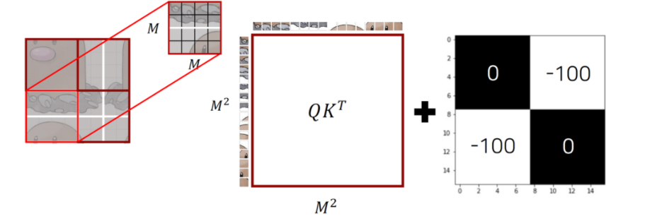
• 첫 번째 window 예시
  - Patch들이 flatten되어 들어가고 self-attention이 적용됨
  - $\small QK^T$ matrix에 attention mask($\small M^2\times M^2$)를 씌우면 원래 인접한 이미지들 부분에서는 mask가 0이고, 인접하지 않은 부분에서는 mask가 -100이 됨을 확인할 수 있음
  

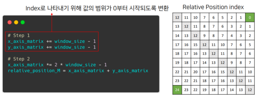
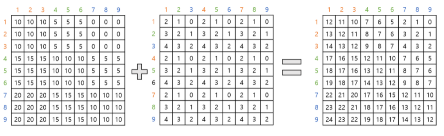
Relative position bias

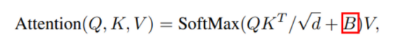
Relative position: $\small [-M+1,\ M-1]$

Bias matrix: $\small \hat B \in \R^{(2M-1) \times (2M-1)}$

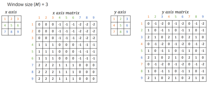
출처: http://dsba.korea.ac.kr/seminar/?mod=document&pageid=1&keyword=swin transformer&uid=1793 고려대학교 DSBA 연구실 Swin Transformer 발표자료

• $\small x-axis\ matrix$ 는 각 행과 열에 해당하는 수의 위치를 왼쪽의 3x3 table에서 구한 뒤, 두 수 위치의 행 차이에 해당하는 값 표기 ex) 1과 7 은 각각 1행과 3행이므로, 1과 7의 교점에 1-3=-2 표기
  
• $\small y-axis\ matrix$ 는 각 행과 열에 해당하는 수의 위치를 왼쪽의 3x3 table에서 구한 뒤, 두 수 위치의 행 차이에 해당하는 값 표기 ex) 3과 5는 각각 3열과 2열이므로, 3과 5의 교점에 3-2=1 표기
  

출처: http://dsba.korea.ac.kr/seminar/?mod=document&pageid=1&keyword=swin transformer&uid=1793, 고려대학교 DSBA 연구실 Swin Transformer 발표자료

• Step 1

$\ \ \ \ \ \ \ \ \ \ \ \ \ \ \ \ \ \ \ \small x-axis\ matrix$ $\ \ \ \ \ \ \ \ \ \ \ \ \ \ \ \ \ \ \ \ \small\ \ \ \ \ \ \ \ \ \ \ \ \ \ \ \ y-axis \ matrix$

• Step 2
  

$\small x-axis\ matrix$ $\small \ \ \ \ \ \ \ y-axis \ matrix$ $\small \ \ \ \ \ \ \ \ \ \ \ \ \ \ \ \ \ relative \ position\ matrix$

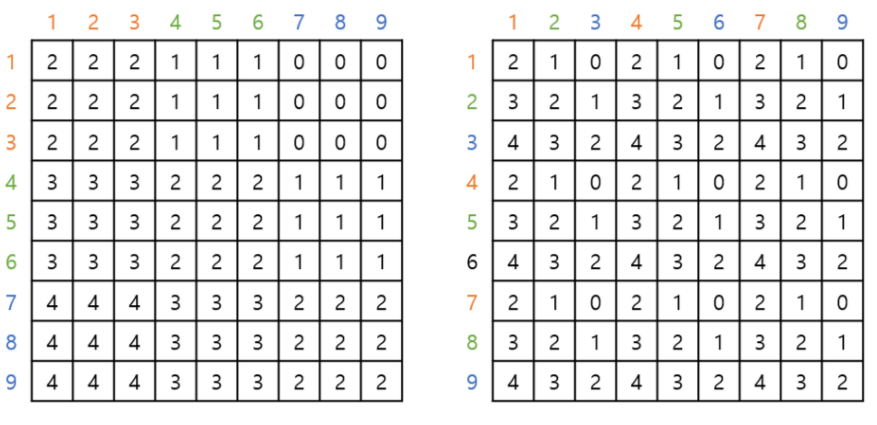
$\small \hat B \in \R^{(2M-1) \times (2M-1)}$ 이므로 $\small 2M-1=5$ , 즉 $\small 5 \times 5$ matrix가 생성

: relative position matrix 내부 값 0~24

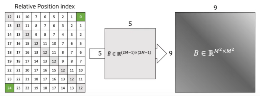
출처: http://dsba.korea.ac.kr/seminar/?mod=document&pageid=1&keyword=swin transformer&uid=1793, 고려대학교 DSBA 연구실 Swin Transformer 발표자료

각 Matrix에 해당하는 값을 $\small \hat B$ 에서 조회하여 $\small B\in \R^{M^2\times M^2}$ 생성: Bias term

Bias matrix는 위 연산에서 $\small qk^T\over \sqrt D$에 더해지므로, 같은 차원을 가져야함 → $\small qk^T\over \sqrt D$: $\small (N_p+1)\times (N_p+1)$

Class token 없을 시 $\small M^2=N_p+1$

• Positional embedding을 모든 token마다 하는 것이 아닌, look up table($\small \hat B$) 를 만들고, relative한 위치를 계산해서 적용하는 방법
• 윈도우 내부의 각 feature이 개별적인 값을 가지도록 설정한 뒤, 지정된 값을 찾아서 position 정보 추가
• 실제로 이후에 일반적인 positional embedding을 추가해 보았을 때, 성능이 하락됨.
• 위의 그림에서는 $\small 9\times 9$이 window, $\small 3\times 3$가 patch

3.3 Architecture Variants

https://openaccess.thecvf.com/content/ICCV2021/papers/Liu_Swin_Transformer_Hierarchical_Vision_Transformer_Using_Shifted_Windows_ICCV_2021_paper.pdf

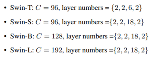
• 기본 모델은 Swin-B. Model size와 계산 복잡도를 각각 0.5배, 0.25배, 2배 한 Swin-S와 Swin-L, Swin-L
• Swin-T와 Swin-S의 계산 복잡도는 각각 ResNet-50, ResNet-101과 유사함

4. Experiments

• ImageNet-1K: Classification
• COCO: Object detection
• ADE20K: Sementic Segmentation

: 위의 3가지 데이터셋에 대해 실험

4.1. Image Classification on ImageNet-1K

Regular ImageNet-1K

• 1.28M training, 50k validation
• AdamW optimizer, 300 epoch
• 초기 20회는 linear warm up 이후에 Cosine decay lr-scheduler, Weight decay 0.05 :→ Linear warmup: 매우 작은 learning rate로 출발해서, weight이 어느정도 안정화시키는 방법으로 0.00에서 출발하여 초기 lr인 0.001까지 linear하게 증가하는 방식을 이용한다.
  
• Batch size 1024, 초기 learning-rate 0.001

Pre-training on ImageNet-22K and fine tuning on ImageNet-1K

• 1.42M training
• Pre-training
  • AdamW optimizer, 90 epoch
  • 초기 5회 linear warm up 이후 linear decay lr-scheduler, Weight decay 0.01
  • Batch size 4096, 초기 learning-rate 0.001
• Fine Tuning
  • AdamW optimizer, 30 epoch
  • Batch size 1024
  • Constant learning rate: 10$\small ^{-5}$
  • Weight decay: 10$\small ^{-8}$

Results

https://openaccess.thecvf.com/content/ICCV2021/papers/Liu_Swin_Transformer_Hierarchical_Vision_Transformer_Using_Shifted_Windows_ICCV_2021_paper.pdf

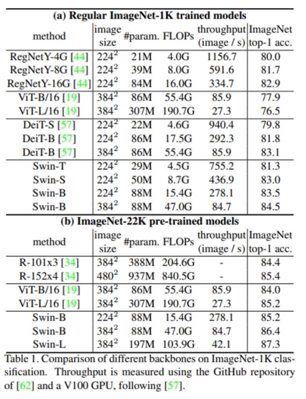
• Swin-B, Swin-L 의 경우 이전의 ViT 기반 모델들에 비해 성능이 향상된 것을 확인할 수 있음
• 기존 ViT에 비해 더 적은 파라미터로 더 좋은 성능을 보여줌
• Deit와 유사한 파라미터 수를 가지지만 Swin transformer에서 더 좋은 성능을 보여줌
• CNN 모델들에 비해 성능과 학습 속도간의 trade-off가 더 작음 (arxiv 논문에는 efficientnet과의 비교가 있는데, CVPR 홈페이지에서 찾은 논문에는 없음)
  

4.2. Object Detection on COCO

• Cascade Masked R-CNN, ATSS, RepPointsv2, Sparse R-CNN 의 4개 framework에 대해 동일 조건으로 실험 진행
  • Multi scale training: 입력 이미지의 짧은 부분 해상도가 480에서 800사이가 되도록 resize
  • AdamW optizmier. 초기 learning rate 0.0001, weight decay 0.05
  • Batch size 16, 36 epochs

https://openaccess.thecvf.com/content/ICCV2021/papers/Liu_Swin_Transformer_Hierarchical_Vision_Transformer_Using_Shifted_Windows_ICCV_2021_paper.pdf

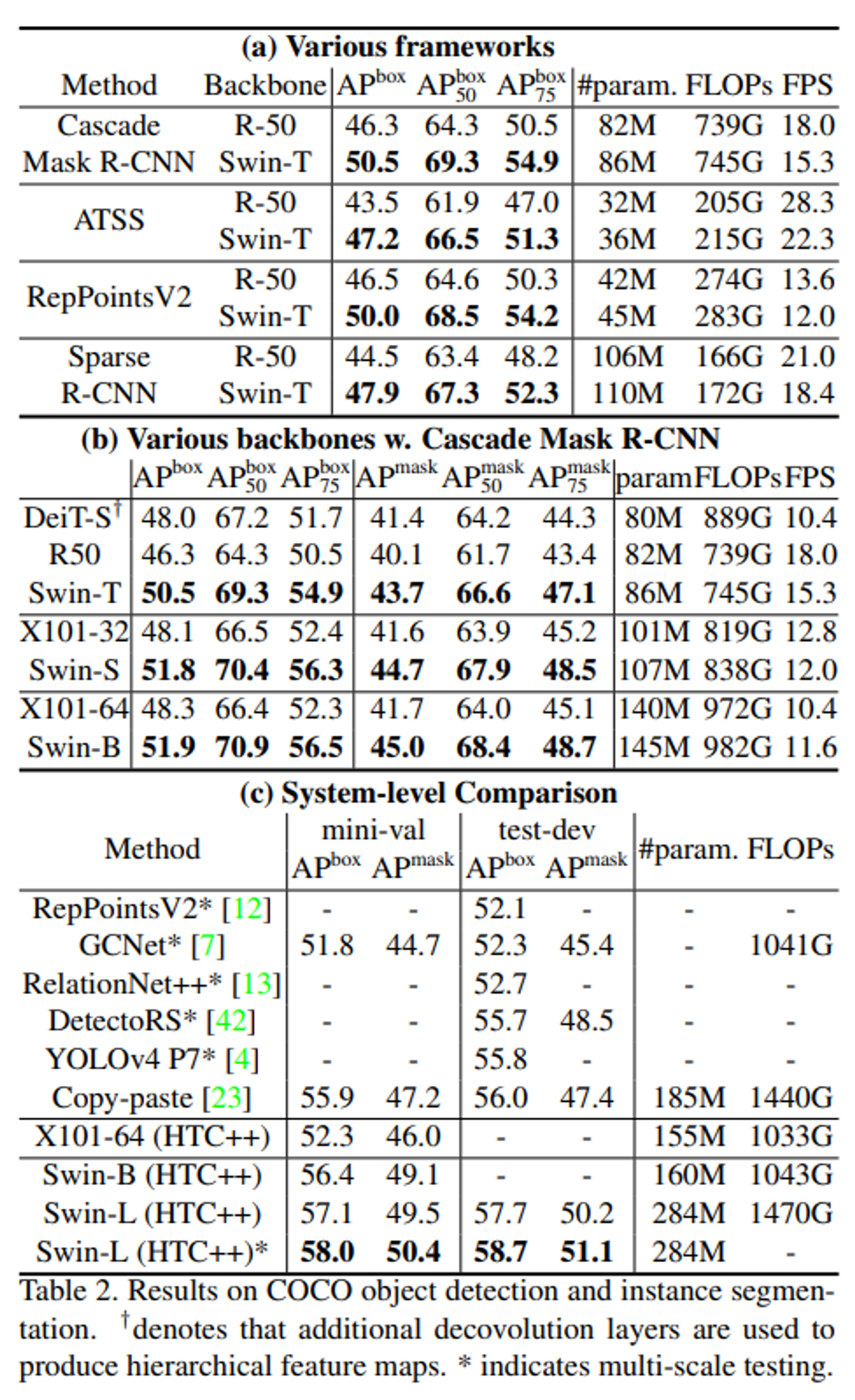
• Resnet 50과 비교해 보았을 때 3.4~4.2 가량의 box AP 차이
• 기존 모델들에 비해 높은 box-AP

4.3 Semantic Segmentation on ADE20K

• 20k training, 2k validation, 3k test로 진행
• UperNet을 base framework로 사용

https://openaccess.thecvf.com/content/ICCV2021/papers/Liu_Swin_Transformer_Hierarchical_Vision_Transformer_Using_Shifted_Windows_ICCV_2021_paper.pdf

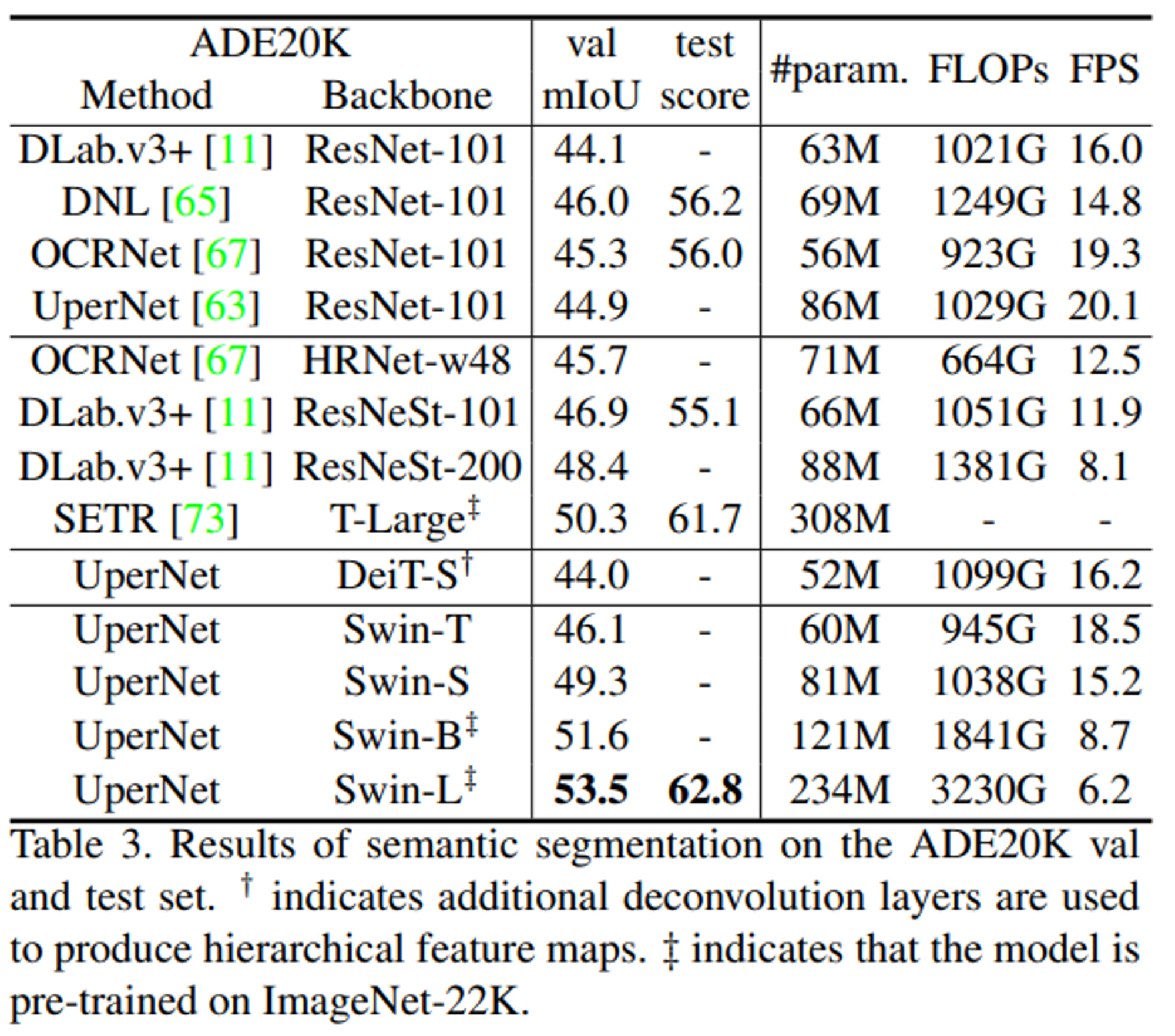
• 기존 Upernet에 backbone로 CNN 기반인 ResNet을 넣었을 때 보다 높은 성능이 기록됨

4.4 Ablation Study

Shifted Window, Relative position bias에 따른 결과 변화

https://openaccess.thecvf.com/content/ICCV2021/papers/Liu_Swin_Transformer_Hierarchical_Vision_Transformer_Using_Shifted_Windows_ICCV_2021_paper.pdf

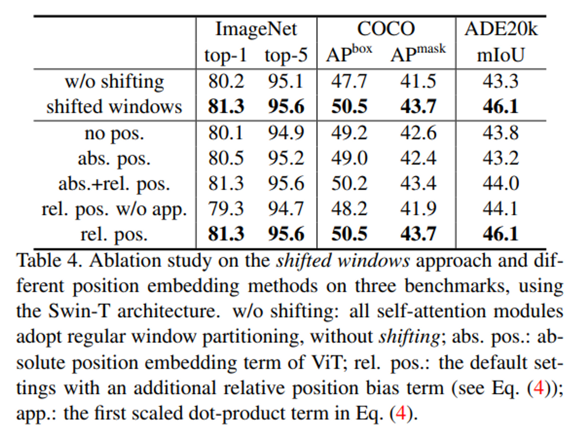
• Shifted window를 적용했을 때 더 좋은 결과를 보임
• Relative position bias를 단독으로 적용했을 때 가장 좋은 결과를 보임
• 특히 Sementic segmentation에서 높은 향상을 관찰할 수 있음 → Dense prediction task에서 position에 대한 중요도가 높으므로 관련 결과가 나왔다고 예상할 수 있음
  

Window 적용 방법에 따른 속도 변화

https://openaccess.thecvf.com/content/ICCV2021/papers/Liu_Swin_Transformer_Hierarchical_Vision_Transformer_Using_Shifted_Windows_ICCV_2021_paper.pdf

• Shifted Window와 Sliding Window 사이 속도 차이가 매우 큰 것을 확인할 수 있음

Window 적용 방법에 따른 성능 변화

https://openaccess.thecvf.com/content/ICCV2021/papers/Liu_Swin_Transformer_Hierarchical_Vision_Transformer_Using_Shifted_Windows_ICCV_2021_paper.pdf

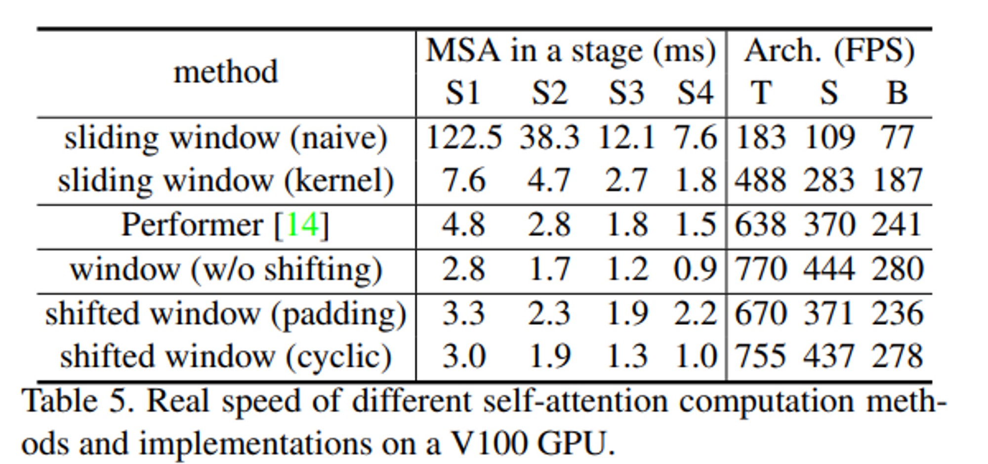
• 성능 면에서는 차이가 거의 없지만, 앞서 본 것 처럼 더 빠른 속도로 동일한 성능을 낼 수 있다는 점에서 의의가 있음

5. Reference

[1]. Ze Liu, Yutong Lin, Yue Cao, Han Hu, Yixuan Wei,
Zheng Zhang, Stephen Lin, and Baining Guo. Swin transformer: Hierarchical vision transformer using shifted windows. arXiv preprint arXiv:2103.14030, 2021

[2]. 고려대학교 DSBA 연구실 Swin Transformer 발표자료

http://dsba.korea.ac.kr/seminar/?mod=document&pageid=1&keyword=swin transformer&uid=1793

[3]. Swin Transformer 논문리뷰

https://pajamacoder.tistory.com/18