1. 탐색적 데이터 분석 EDA
EDA?
- 데이터 그 자체를 보는 눈
데이터를 분석하는 기술적 접근은 매우 많다.
데이터 그 자체만으로부터 인사이트를 얻어내는 접근법! - 통계적 수치나 numpy/pandas등으로 알 수 있다.
EDA의 Process
- 분석의 목적과 변수 확인
- 데이터 전체적으로 살펴보기
- 데이터의 개별 속성 파악하기
EDA with example - Titanic
https://www.kaggle.com/c/titanic/data
1. 분석의 목적과 변수 확인
- 분석의 목적확인
살아남은 사람들은 어떤 특징을 가지고 있었을까? - 변수확인
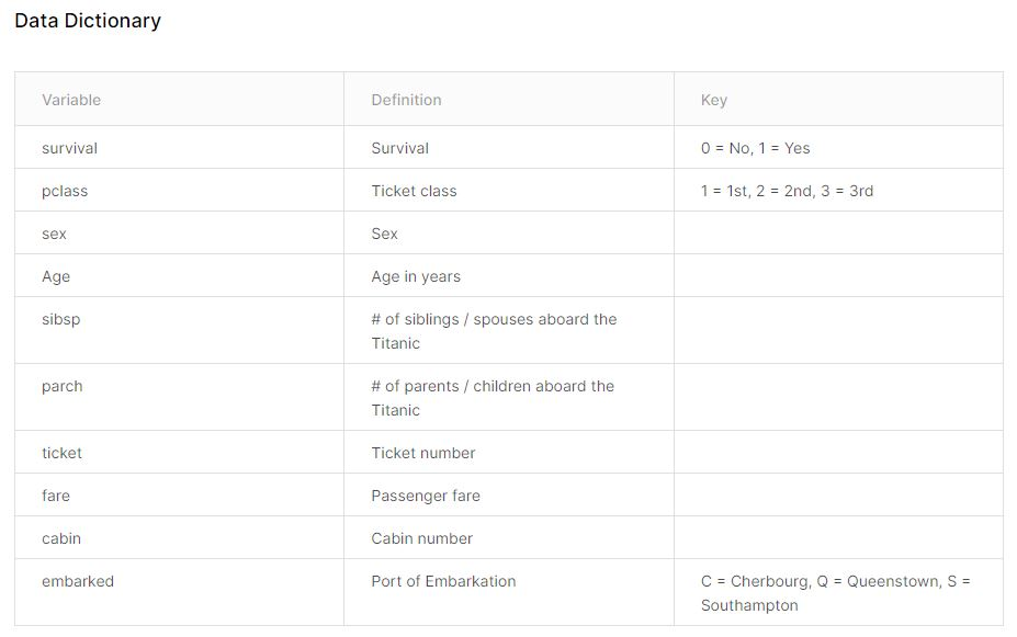
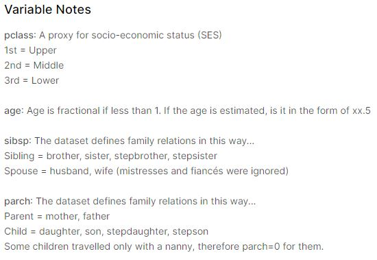
변수(variable)는 10개 있다.
key는 숫자로 인코딩 되었다면 그 뜻
Definition 변수의 의미
데이터 살펴보기
# 라이브러리 불러오기
import numpy as np
import pandas as pd
import matplotlib.pyplot as plt
import seaborn as sns

%matplotlib inline

# 데이터 불러오기, 동일경로
titanic_df = pd.read_csv("./train.csv")

# 상위 5개 데이터 확인

titanic_df.head(5)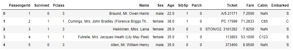
# 각 column의 데이터 타입 확인

titanic_df.dtypes

->
PassengerId      int64
Survived         int64
Pclass           int64
Name            object
Sex             object
Age            float64
SibSp            int64
Parch            int64
Ticket          object
Fare           float64
Cabin           object
Embarked        object
dtype: object
2. 데이터 전체적으로 확인하기
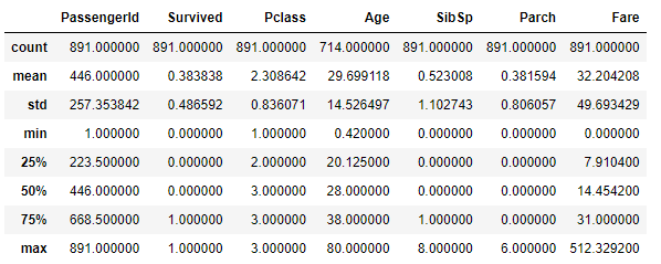
- 데이터 전체 정보를 얻는 함수 :
.describe()
-> 수치형 데이터에 대한 요약만을 제공
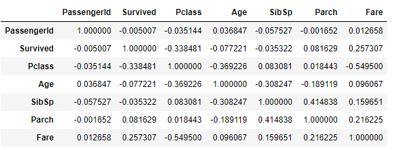
상관계수 확인
.corr()Correlation is NOT Causation
상관성 : A up, B up, ...
인과성 : A -> B
상관관계로부터 인과성을 증명하긴 매우 어렵다. 구분해서 사용해야함!
결측치 확인
- 결측치 확인은 매우 중요하다, 어떻게 사용해야하는지 생각해야하기 때문이다.
(Age, Cabin, Embarked에서 결측치를 발견!) .isnull()
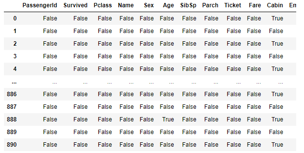
titanic_df.isnull().sum()

->
PassengerId      0
Survived         0
Pclass           0
Name             0
Sex              0
Age            177
SibSp            0
Parch            0
Ticket           0
Fare             0
Cabin          687
Embarked         2
3. 데이터의 개별 속성 파악하기
survived Column
# 생존자, 사망자 명수는?

titanic_df['Survived'].sum()
-> 342

titanic_df['Survived'].value_counts()
->
0    549
1    342
# 생존자 수와 사망자 수를 Barplot으로 그려보기 sns.countplot()
sns.countplot(x ='Survived', data=titanic_df)
plt.show()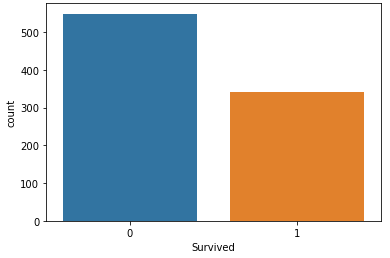
Pclass
# Pclass에 따른 인원 파악
titanic_df[['Pclass','Survived']]
->
 Pclass Survived
0	3	0
1	1	1
2	3	1
3	1	1
4	3	0
...	...	...
886	2	0
887	1	1
888	3	0
889	1	1
890	3	0

#Pclass별 탑승인원
titanic_df[['Pclass','Survived']].groupby('Pclass').count()
->
	Survived
Pclass
1	216
2	184
3	491

# 생존자 인원?
titanic_df[['Pclass','Survived']].groupby('Pclass').sum()
->

  Survived
Pclass
1	136
2	87
3	119

# 생존률?
titanic_df[['Pclass','Survived']].groupby('Pclass').mean()
	Survived
Pclass
1	0.629630
2	0.472826
3	0.242363

# 히트맵 활용
sns.heatmap(titanic_df[['Pclass','Survived']].groupby('Pclass').mean())
plt.show()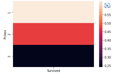
Sex
titanic_df[['Sex', 'Survived']]
->
	Sex	Survived
0	male	0
1	female	1
2	female	1
3	female	1
4	male	0
...	...	...
886	male	0
887	female	1
888	female	0
889	male	1
890	male	0

titanic_df.groupby(['Survived','Sex']).count()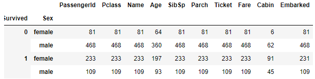
titanic_df.groupby(['Survived','Sex'])['Survived'].count()
->
Survived  Sex
0         female     81
          male      468
1         female    233
          male      109
# sns.catplot
sns.catplot(x='Sex', col='Survived', kind='count',data=titanic_df)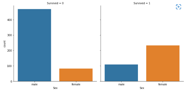
Age
- 결측치 존재
titanic_df.describe()['Age']
->
count    714.000000
mean      29.699118
std       14.526497
min        0.420000
25%       20.125000
50%       28.000000
75%       38.000000
max       80.000000
# survived 1, 0과 Age의 경향성
# figure(도면) -> axis(틀) -> plot
fig, ax = plt.subplots(1, 1, figsize=(10,5))
sns.kdeplot(x=titanic_df[titanic_df.Survived==1]['Age'],ax=ax)
sns.kdeplot(x=titanic_df[titanic_df.Survived==0]['Age'],ax=ax)
plt.legend(['Survived', 'Dead'])
plt.show()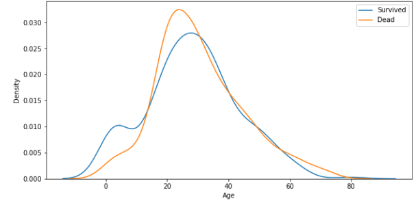
# subplots를 사용하지 않아도 그래프를 중복해서 그릴 수 있다.
plt.figure(figsize=(10,6))
sns.kdeplot(x=titanic_df[titanic_df.Survived==1]['Age'])
sns.kdeplot(x=titanic_df[titanic_df.Survived==0]['Age'])
plt.legend(['Survived', 'Dead'])
plt.show()
Appendix I.Pclass + Sex vs Survived
# 복합적인 요소에 대해 분석 진행
# 성별과 pclass, survived
# 각 점은 추정치

sns.catplot(x='Pclass', y='Survived', hue='Sex', kind='point',data=titanic_df)
plt.show()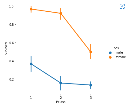
Appendix II.Pclass + Age vs Survived
# Age graph with pclass

titanic_df['Age'][titanic_df.Pclass==1].plot(kind='kde')
titanic_df['Age'][titanic_df.Pclass==2].plot(kind='kde')
titanic_df['Age'][titanic_df.Pclass==3].plot(kind='kde')
plt.legend(['1st','2nd','3rd'])
plt.show()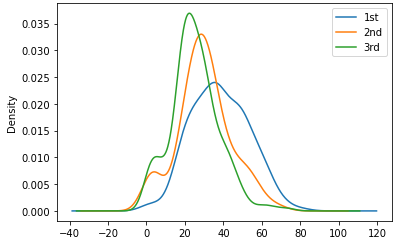
Mission : It's Your Turn!
1. 본문에서 언급된 Feature를 제외하고 유의미한 Feature를 1개 이상 찾기
- Hint : Fare? Sibsp? Parch?
2. Kaggle에서 Dataset을 찾고, 이 Dataset에서 유의미한 Feature를 3개 찾고 시각화
함께보면 좋은 라이브러리
- numpy
- pandas
- seaborn
- matplotlib
Hint!!
1.데이터 뽑아보기
- 각 데이터는 어떤 자료형을 가지고 있나?
- 데이터에 결측치는 없나? -> 있다면 어떻게 메꿔줄지?
- 데이터의 자료형을 바꿔줄 필요가 있나? -> 범주형의 One-hot encoding
2.데이터에 대한 가설을 세우기
- 가설을 개인의 경험에 의해서 도출되어도 상관이 없다.
- 가설은 명확할 수록 좋다.
- 타이타닉에서 성별과 생존률은 상관이 있을 것이다.
3.가설을 검증하기 위한 증거를 찾아본다.
- 이 증거는 한 눈에 보이지 않을 수 있다. 여러 테크닉을 써줘야 한다.
.groupby()를 통해서 그룹화된 정보에 통계량을 도입하기.merge()를 통해서 두개 이상의 dataframe을 합쳐본다- 시각화를 통해 일목요연하게 보여준다.

초보 컴공