-
원문
ICML: https://icml.cc/virtual/2025/poster/43564
Openreview: https://openreview.net/forum?id=xnEv5pq4cB
1. Introduction
- 기존 연구 문제점
- LLM serving workload heterogeneity
- 두 페이즈로 나뉜다.
- The prefill phase: compute-bound, 1 step
The decoding phase: memory-bound, step-by-step - 이렇게 다른 워크로드를 homogeneous GPU로 서빙하는 것은 비효율적일 수 있다.
- LLM serving workload heterogeneity
주요 질문
본 논문의 주요 질문은 두 가지이다.
- Q1. LLM serving에 있어서 heterogeneous GPU가 homogeneous GPU보다 나은 cost-efficiency를 제공할 수 있나?
- Q2. 만약 그렇다면, 어떻게 heterogeneous GPU가 더 나은 cost-efficiency를 제공할 수 있나?
논문에서 문제시한 것이 ‘homogeneous GPU의 LLM serving 능력 부족’이므로, 이 논문의 contribution은 이 질문에 대한 답변과 동치된다.
Contribution
-
Q1. LLM serving에 있어서 heterogeneous GPU가 homogeneous GPU보다 나은 cost-efficiency를 제공할 수 있나? (판별 가능?)
-
A1(The first contribution). 벤치마킹을 통해, 무엇이 cost-efficiency인지 판별할 수 있는 세 가지 지표를 발견했다. (판별 기준 제시.)
- GPU composition:
GPU 수 & 종류.
Resource utilization, latency, overall performance에 영향을 줌. - Deployment configuration:
배포 모델 수 & parallelism strategy.
Model, workload, GPU type에 영향을 받음.
System efficiency에 영향을 줌. - Workload assignment:
replicas→vary config→vary workload→vary resource→전략적 할당 필요
- GPU composition:
-
Q2. 만약 그렇다면, 어떻게 heterogeneous GPU가 더 나은 cost-efficiency를 제공할 수 있나?
-
A2(The second contribution). 새로운 LLM serving framework를 디자인했다. 이는 heterogeneous GPU가 (클라우드 플랫폼의 자원을 이용하여) 더 나은 cost-efficiency를 제공할 수 있다.
제약 설정
- Real-time GPU availability 제약이 있다. (논문에서는 cloud platform에서의 serving을 전제하고 있다.)
- User-defined price budget 제약이 있다.
- A1에 나온 조건을 모두 충족하는 GPU 골라 쓰면 문제 해결 아닌가?
→ 위 제약때문에 안 된다.
결과
- Throughput: 평균 20% 최대 41% 향상
(혹은)
- Latency: 평균 20% 최대 54% 감축
2. Background
LLM inference phase
- The prefill phase
- 사용자가 입력한 프롬프트를 한번에 병렬처리하여 KV 캐시 생성
- compute-bound(parallelized calculation for all input tokens), 1 step
- The decoding phase
- 토큰 출력을 autoregressive하게 생성하는 과정
- memory-bound(얼마나 빠르게 KV 캐시가 로드되는지 등), step-by-step
Workload heterogeneity
- LLM의 task에 따라 input & output token 길이가 상이한 것 → 요구하는 리소스가 이에 따라 달라짐
- The decoding phase (메모리 바운드) 예시: WildGPT dataset 평균 인풋 496, 아웃풋 510
- The prefill phase (컴퓨트 바운드) 예시: Azure-Trace dataset 평균 인풋 2455, 아웃풋 18
Heterogeneous LLM serving
- HexGen
- Asymmetric partitioning & scheduling techniques
- GPU allocation을 bin-packing problem으로 정의하고, cost efficiency를 최적화함
- Helix
- GPU & network connection optimization 문제를 max-flow 문제로 정의
- MILP 통해서 optimal model deployment 결정
- 선행연구 한계점
- GPU composition ❌
Predefined GPU cluster만 상정함. - 제약 반영 ❌
Real-time GPU availability, User-defined price budget 고려 안 함 - Workload assignment ❌
단일(uniform) 워크로드만 상정함.
- GPU composition ❌
LLM serving optimization
-
QLM
- SLO(서비스 수준 목표)-aware serving, Multi-node optimization
-
Sarathi-Serve
- 배칭 최적화: prefill chunking to mitigate interference between the prefill and decoding stages
-
Vidur
- An accurate simulator for deployment tuning
-
선행 연구와의 차별점
- 주안점: heterogeneous, cloud env, cost-efficient
3. Observation and Opportunity
: The first contribution
Benchmarking settings
- Workload 9종류(3*3)
- ShareGPT (Zheng et al.), WildGPT (Zhao et al.), and Azure-Trace datasets (Patel et al., 2024)
- Average input token length: {2455, 824, 496}, (long≥512)
- Average output token length: {510, 253, 18}, (long≥128)
- Model 2종류
- Llama3-8B
- Llama3-70B
- GPU 6종류
- A6000, A40, L40, A100, H100, 4090
- Deployment configuration 다 다름
- Benchmarking metrics
- request throughput / unit price
- total cost (w/ various latency percentiles) == latency time * unit price
- unit price는 GPU cost를 의미함
Observation-1
GPU composition
: Heterogeneous GPUs are well-suited for managing model and workload diversity in LLM serving
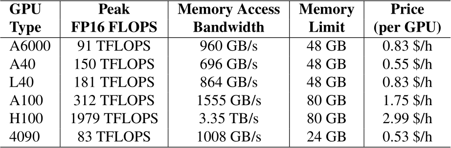
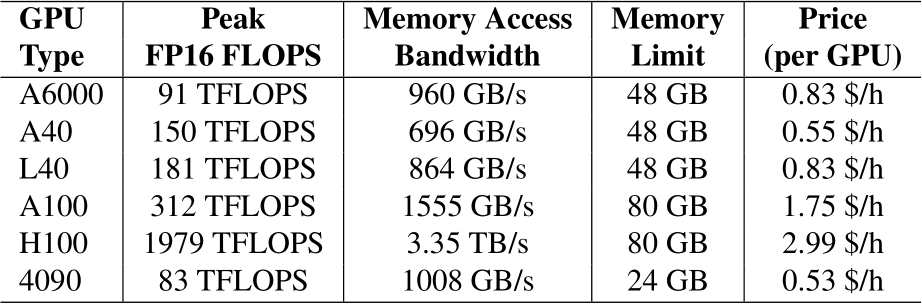
- The A100 and H100 GPUs (data center GPUs)
- Llama3-70B model, compute-intensive workloads 굿
- 메모리는 주로 underutilized
- The A6000, A40, and L40 GPUs (workstation GPUs)
- Llama3-70B model, memory-intensive workloads 굿
- (data center GPUs 대비)
memory bandwidth / unit price 평균 1.2배 이상
memory capacity / unit price 평균 1.8배 이상
- The 4090 GPUs (consumer GPUs)
- Llama3-8B model, performance 굿
- 모델 작음 → compute, memory resource 적게 요구함
- (data center GPUs 대비)
memory bandwidth / unit price 약 1.9배 이상
- 결론
- performance and cost-efficiency 향상을 위해서
특정 workloads, models에 맞는
GPU 타입을 고르는 것이 중요하다. - cost-efficiency performance를 최대 2.27배 향상
- performance and cost-efficiency 향상을 위해서
Observation-2
Deployment configuration
: Optimal deployment configurations are crucial for maximizing cost-efficiency across models, workloads, and GPU types.
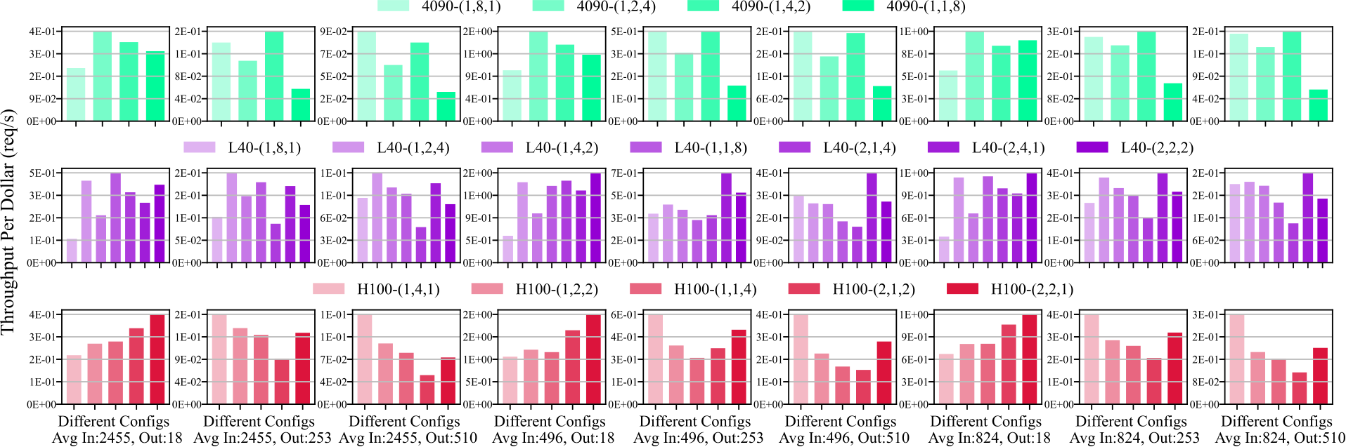
GPU-(tensor parallelism (TP), pipeline parallelism (PP), and data parallelism (DP))
- Optimal configs가 workload에 따라 다름 (동일 GPU 타입)
- Optimal configs가 GPU 타입에 따라 다름 (동일 workload)
- Optimal configs가 모델 타입에 따라 다름
- 결론
- system performance 향상을 위해서는
특정 workloads, models, GPU type에 맞는
Configuration을 고르는 것이 중요하다. - system performance를 최대 2.61배 향상
- system performance 향상을 위해서는
Observation-3
Workload assignment
: The workload assignment should be co-optimized with heterogeneous GPU composition and deployment configurations
Two key objectives:
-
특정 요청의 리소스 요구사항에 가장 잘 매치되는 GPU 타입 & Configs를 찾기
GPU composition에 더해 Deployment configuration 맞추는 것이 중요
-
GPUs간 workloads 분산하기(과부하 방지)
전체의 효율을 위해 sub-optimal한 선택을 할 수 있어야 함
Constraints
: Appropriate resource scheduling is crucial under limited resources and budget constraints
- A1에 나온 조건을 모두 충족하는 GPU 골라 쓰면 문제 해결 아닌가?
→ 아래 제약때문에 안 된다.
-
Real-time GPU availability 제약이 있다. (논문에서는 cloud platform에서의 serving을 전제하고 있다.)
i.e. A40 availability on RunPod and Vast.ai 는 시간에 따라 3~16, 0~32개 사용 가능.
-
User-defined price budget 제약이 있다.
돈이 없어서 optimal GPU를 각 workload에 할당하지 못할 수 있다.
- 그럼 어떻게 함?
→ effective scheduling algorithm으로 최대한 제약조건 아래에서 최고의 serving을 해보자
Opportunities
: Optimization of heterogeneous GPU deployment for cost-efficient LLM serving
- Determining the optimal heterogeneous GPU composition (observation-1)
- Selecting the most effective deployment configurations (observation-2)
- Implementing the most appropriate workload assignment (observation-3)
→ deliver a comprehensive LLM serving plan that meets user requirements, adapts to cloud environment constraints, and maximizes cost-efficiency (constraints)
4. Scheduling Algorithm
4.1. Problem Formulation
- Plan 구성물
- GPU composition
- Deployment configurations
- Workload assignment
- Plan Objective
- min the overall makespan (for processing all incoming workloads)
- max cost-efficient ****LLM serving solution (under the specified budgetary and resource constraints)
4.2. Simple Example
Experiment setup
- GPU { , , }
GPU type prices($/h) available unit 4 2 2 2 2 2 - Workload {, }
- : simultaneously with 80 total requests()
- : simultaneously with 20 total requests()
- Throughput
1.0 1.2 0.9 0.9 0.3 0.5
Case 1: GPU composition
- 각 모델이 Workload {, }를 수행한다 가정했을 때
| budget == 8$/h | composition 1 | composition 2 |
|---|---|---|
| GPU composition | { , , } | { , , } |
| total throwput | (2.2, 2.6) | (2.8, 3.0) |
| processing time | 44.05s | 35.24s |
→ 20% 속도 향상
Case 2: Deployment configuration
| 1.0 | 1.2 | |
| 0.9 | 0.9 | |
| 0.3 | 0.5 | |
| (TP) | 2.4 | 1.5 |
| budget == 8$/h | composition 1 | composition 2 | composition 2 (conf) |
|---|---|---|---|
| GPU composition | { , , } | { , , } | { , -} |
| total throwput | (2.2, 2.6) | (2.8, 3.0) | (3.4, 2.7) |
| processing time | 44.05s | 35.24s | 30.94s |
→ 약 14% 속도 향상
Case 3: Workload assignment
| budget == 8$/h | composition 1 | composition 2 | composition 2 (conf) | composition 2 (conf)(WA) |
|---|---|---|---|---|
| GPU composition | { , , } | { , , } | { , -} | { , -} |
| Workload assignment | {(1, 1),(1, 1),(1, 1)} | {(1, 1),(1, 1),(1, 1)} | {(1, 1),(1, 1)-(1, 1)} | {(0.45, 3),(1.275, 0)-(1.275, 0)} |
| total throughput | (2.2, 2.6) | (2.8, 3.0) | (3.4, 2.7) | (3.51, 3.6) |
| processing time | 44.05s | 35.24s | 30.94s | 28.67s |
→ 약 8% 속도 향상
4.3. MILP Formulation
- {GPU composition, Deployment configurations, Workload assignment}이 중요하다는 건 알겠다.
- 그런데 어떻게 최적의 값을 구할 것인가? → MILP 사용
Configurations
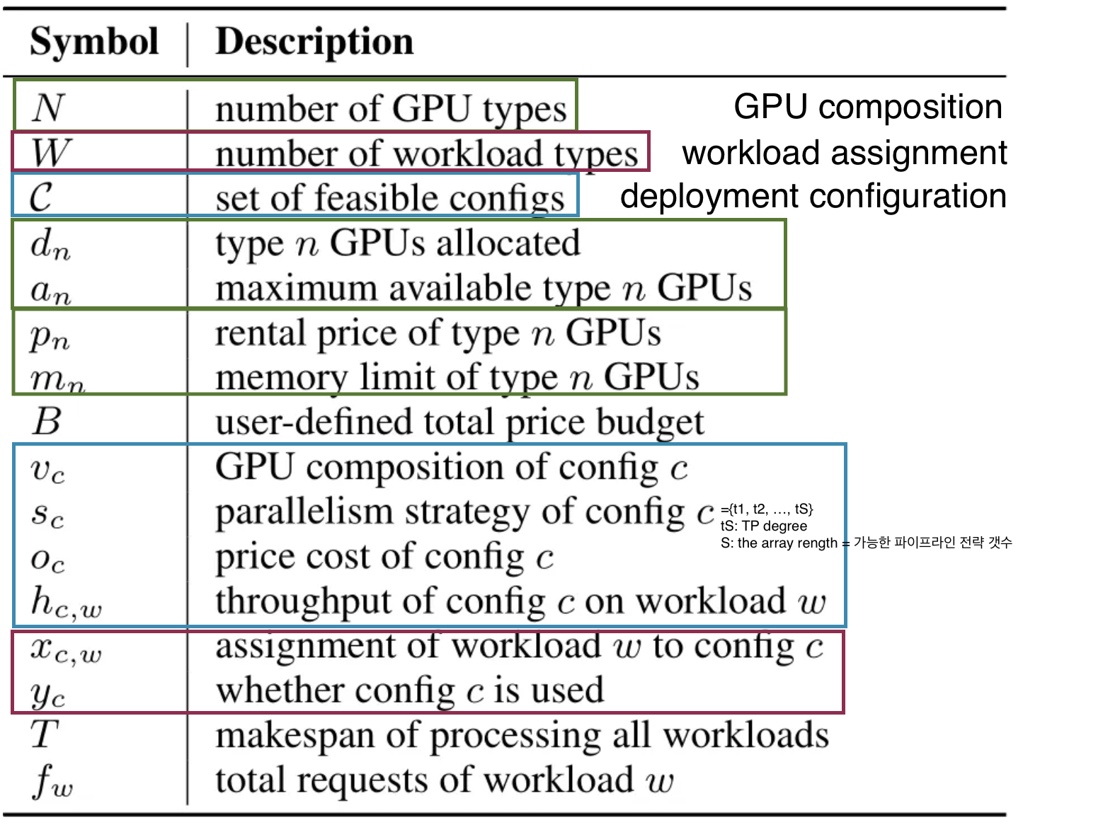
GPU composition
- D = [ d1, d2, . . . , dN ], dn ≥ 0, vector
- A = [ a1, a2, . . . , aN ], 0 ≤ dn ≤ an, vector
- pn = GPU type n의 가격
- mn = GPU type n의 메모리 용량
Deployment configuration
- c ∈ C = 서빙 플랜, (vc, sc, oc, hc,w)로 구성됨
- S = array length, 가능한 파이프라인 스테이지 갯수
- sc = {t1, t2, . . . , tS}, ts = s번째 스테이지의 TP degree, sc의 합은 dn의 합과 같음
- hc,w의 메트릭은 one-time profiling 사용. (Appendix L)
Workload assignment
- w ∈ {1, 2, . . . , W}
- fractional assignment: a fraction xc,w ∈ [0, 1]
Budget and GPU constraints


- GPU 상한과 budget 상한을 넘지 말아야 한다는 것을 수식으로 표현함.
Optimization objective
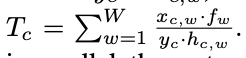
일 때, T를 최소화하는 것이 목적이다.
MILP formulation
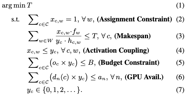
Complexity analysis
이론상 worst-case

즉, configuration 후보 수의 숫자에 따라 기하급수적으로 복잡도가 증가한다.
Other constraints and heuristics
(따라서?) 서치 스페이스를 줄이기 위한 추가 제약과 휴리스틱을 도입했다.
- 메모리 제한 강화 → 불충분한 gpu 메모리를 사용하는 후보 configuration 제거
- 연결 끊긴 gpu 포함하는 configuration 제거
- TP 단일 머신 제한: 미준수 configuration 제거
- non-uniform PP layer partitioning (based on memory allocation) 허용
Appendix D
Binary search
MILP로 large-scale problems를 풀기에는 너무 오랜 시간이 걸리기 때문에, 이를 가속하기 위해 binary-search-on-T를 도입했다.
T를 직접적으로 최소화하는 대신, iteratively T의 후보군 중에 유효한 플랜이 존재하는지를 체크했다. (휴리스틱한 상한/하한을 기준삼았다고 함. 본문에서는 ‘reasonable’이라고 표현했지만)
Appedix F
Extension to multiple LLM serving
- 성취: simultaneously serving both Llama3-8B and Llama3-70B model
- 이를 위해, model-type dimension을 도입했다.
- variables와 constraints를 결정
- 이를 통해 workload assignments, memory requirements, and other constraints를 확인할 수 있었다.
Appen
5. Experiments
논문 본문 보는 게 나음
6. Conclusion
목적
- Why & How / heterogeneous cloud resources가 / LLM serving에 있어 / cost efficiency?
- Q1. LLM serving에 있어서 heterogeneous GPU가 homogeneous GPU보다 나은 cost-efficiency를 제공할 수 있나?
- Q2. 만약 그렇다면, 어떻게 heterogeneous GPU가 더 나은 cost-efficiency를 제공할 수 있나?
방법
- {heterogeneous GPU / LLM serving / cost efficiency} 벤치마킹
- 새로운 스케줄링 알고리즘 제시
결과
- 기존 방법보다 나은 것으로 밝혀짐
관련자료
- LLM inference phase
- 두 페이즈와 배칭에 대한 설명 https://huggingface.co/blog/tngtech/llm-performance-prefill-decode-concurrent-requests
- 전반적으로 다룸(배칭, 캐싱, parallelization, 어텐션 메커니즘 최적화, 모델 최적화, 서빙 전략) https://developer.nvidia.com/ko-kr/blog/mastering-llm-techniques-inference-optimization/
- 두 페이즈와 배칭에 대한 설명 https://huggingface.co/blog/tngtech/llm-performance-prefill-decode-concurrent-requests
- Heterogeneous LLM serving
- HexGen
https://arxiv.org/abs/2311.11514https://www.themoonlight.io/ko/review/hexgen-2-disaggregated-generative-inference-of-llms-in-heterogeneous-environment - Helix
https://arxiv.org/abs/2406.01566https://www.themoonlight.io/ko/review/helix-serving-large-language-models-over-heterogeneous-gpus-and-network-via-max-flow
- HexGen
- LLM serving optimization
- QLM
https://arxiv.org/abs/2407.00047 - Sarathi-Serve
https://arxiv.org/abs/2403.02310 - Vidur
https://arxiv.org/abs/2405.05465
- QLM
- 기타