기울기 소실 문제와 활성화 함수
오차 역전파는 출력층으로부터 하나씩 앞으로 되돌아가며 각 층의 가중치를 수정하는 방법
가중치를 수정하려면 미분 값, 즉 기울기가 필요하다고 배움
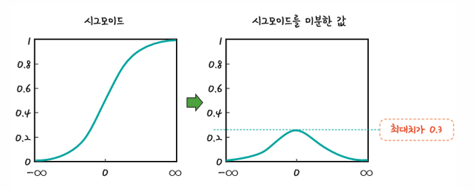
그런데 층이 늘어나면서 기울기가 중간에 0이 되어버리는 기울기 소실(vanishing gradient) 문제가 발생하기 시작
이는 활성화 함수로 사용된 시그모이드 함수의 특성 때문임
아래 그림처럼 시그모이드를 미분하면 최대치가 0.3
1보다 작으므로 계속 곱하다 보면 0에 가까워짐
따라서 층을 거쳐 갈수록 기울기가 사라져 가중치를 수정하기가 어려워지는 것
이를 해결하고자 활성화 함수를 시그모이드가 아닌 여러 함수로 대체하기 시작
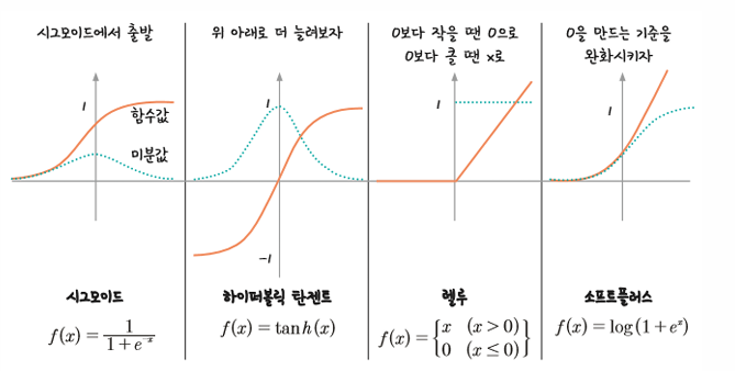
시그모이드 함수의 범위를 -1에서 1 로 확장한 개념인 하이퍼볼릭 탄젠트(tanh)는 미분한 값의 범위가 함께 확장되는 효과를 가져왔음
하지만 여전히 1보다 작은 값이 존재하므로 기울기 소실 문제는 사라지지 않음
토론토대학교의 제프리 힌튼 교수가 제안한 렐루(ReLu)는 시그모이드의 대안으로 떠오르며 현재 가장 많이 사용되고 있는 활성화 함수
렐루는 x 가 0보다 작을 때는 모든 값을 0으로 처리하고, 0보다 큰 값은 x를 그대로 사용하는 방법. 이 방법을 쓰면 x가 0보다 크기만 하면 미분 값이 1 이 됨
따라서 여러 은닉층을 거치며 곱해지더라도 맨 처음 층까지 사라지지 않고 남아있을 수 있음 -> 딥러닝의 발전에 속도가 붙게 됨
속도와 정확도 문제를 해결하는 고급 경사 하강법
경사 하강법은 정확하게 가중치를 찾아가지만, 한 번 업데이트할 때마다 전체 데이터를 미분해야 하므로 계산량이 매우 많다는 단점이 있음
확률적 경사 하강법(SGD)
전체 데이터를 사용하는 것이 아니라, 랜덤하게 추출한 일부 데이터를 사용
일부 데이터를 사용하므로 더 빨리 그리고 자주 업데이트를 하는 것이 가능해짐
모멘텀
경사 하강법과 마찬가지로 매번 기울기를 구하지만, 이를 통해 오차를 수정하기 전 바로 앞 수정 값과 방향(+,-)을 참고하여 같은 방향으로 일정한 비율만 수정되게 하는 방법( 이도에 탄력을 더한다)
AdaGrad
신경망 학습에서 학습률은 중요한 값이다. 이 값이 너무 작으면 학습 시간이 길어지고, 반대로 너무 크면 발산하여 학습이 제대로 이루어 지지 않는다. 학습률을 정하는 효과적인 기술로 학습률 감소가 있다. 이를 이용한 방법이 AdaGrad이다.
즉 학습을 진행하면서 학습률을 점차 줄여가는 방법이다.
Adam
모멘텀은 공이 그릇 바닥을 구르는 듯한 움직임을 보였다. AdaGrad는 매개변수의 원소마다 적응적으로 갱신정도를 조정했다. 위의 두 방법을 융합하여 만든 기법이 Adam 이다.
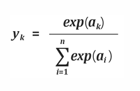
소프트맥스
소프트맥스는 총합이 1인 형태로 바꿔서 계산해 주는 함수
합계가 1 인 형태로 변환하면 큰 값이 두드러지게 나타나고 작은 값은 더 작아짐
이 값이 교차 엔트로피를 지나 [1.,0.,.0.]으로 변화하게 되면 우리가 원하는 원-핫 인코딩 값, 즉 하나만 1이고 나머지는 모두 0인 형태로 전환시킬 수 있음
소프트맥스 함수
소프트 맥스는 클래스 분류 문제를 풀 때 점수 벡터를 클래스 별 확률로 변환하기 위해 흔히 사용하는 함수이다. 각 점수 벡터에 지수를 취한 후, 정규화 상수로 나누어 총 합이 1 이 되도록 계산한다.
출력 총합이 1인 된다는 점은 소프트맥스 함수의 출력을 확률로 해석 할 수 있다.
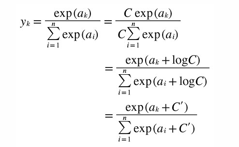
소프트맥스 함수를 구현 할 때 오버플로 문제가 발생 할 수 있다. 소프트맥스 함수는 지수 함수를 사용하는데, 지수 함수는 입력 값에 따라 아주 큰 값을 내뱉는데 이러한 큰 값 끼리 나눗셈을 하면 수치가 불안정해진다 그래서 다음과 같이 소프트맥스 함수 구현 시 수식을 개선하게 된다.
import numpy as np

wsum = np.array([0.9,2.9,4.0])

def softmax(ws):
    exp_a = np.exp(ws)
    sum_exp_a = np.sum(exp_a)
    y = exp_a / sum_exp_a
    return y

def softmax2(ws):
    c = np.max(ws)
    exp_a = np.exp(ws-c)
    sum_exp_a = np.sum(exp_a)
    y = exp_a / sum_exp_a
    return y


output = softmax(wsum)
print(output)
print(output.sum())

output2 = softmax2(wsum)
print(output2)
print(output2.sum())
[0.03269362 0.24157499 0.72573139]
0.9999999999999999
[0.03269362 0.24157499 0.72573139]
1.0
교차 엔트로피
Entropy
정보를 최적으로 인코딩 하기 위해 필요한 bit의 수

오차 함수에는 평균 제곱 오차 계열의 함수 외에도 교차 엔트로피 계열의 함수가 있음
-> 평균 제곱 오차는 수렴하기까지 속도가 많이 걸린다는 단점이 있다
-> 교차 엔트로피는 출력 값에 로그를 취해서, 오차가 커지면 수렴 속도가 빨라지고 오차가 작아지면 속도가 감소하게끔 만든 것
교차 엔트로피는 주로 분류 문제에서 많이 사용
import torch
import torch.nn.functional as F


torch.manual_seed(777)

wsum = torch.randn(3,5,requires_grad=True)
print(wsum)
hypothesis = F.softmax(wsum, dim=1)
print()
print(hypothesis)
print()

y = torch.randint(5,(3,)).long()
print(y)
print()

y_one_hot = torch.zeros_like(hypothesis)
print(y_one_hot)
print()

y_one_hot = y_one_hot.scatter(1,y.unsqueeze(dim=1),1)    #  scatter함수 안 맨앞은 dim 값  마지막 숫자는 채울값
print(y_one_hot)

print(-(y_one_hot * torch.log(F.softmax(wsum, dim=1))).sum(dim=1))
print(-(y_one_hot * torch.log(F.softmax(wsum, dim=1))).sum(dim=1).mean())
print(-(y_one_hot * torch.log_softmax(wsum, dim=1)).sum(dim=1).mean())
print(F.cross_entropy(wsum,y))
tensor([[-0.4015, -0.5934, 1.6885, 0.5554, -0.9433],
[-0.6758, 1.4425, -1.4711, -1.3173, 2.3271],
[ 0.0894, 0.6558, -0.5836, -0.1074, 0.0367]], requires_grad=True)
tensor([[0.0764, 0.0630, 0.6174, 0.1988, 0.0444],
[0.0329, 0.2732, 0.0148, 0.0173, 0.6618],
[0.1983, 0.3494, 0.1012, 0.1629, 0.1882]], grad_fn=<SoftmaxBackward0>)
tensor([3, 0, 0])
tensor([[0., 0., 0., 0., 0.],
[0., 0., 0., 0., 0.],
[0., 0., 0., 0., 0.]])
tensor([[0., 0., 0., 1., 0.],
[1., 0., 0., 0., 0.],
[1., 0., 0., 0., 0.]])
tensor([1.6154, 3.4157, 1.6178], grad_fn=<NegBackward0>)
tensor(2.2163, grad_fn=<NegBackward0>)
tensor(2.2163, grad_fn=<NegBackward0>)
tensor(2.2163, grad_fn=<NllLossBackward0>)예제2
import torch
import torch.nn as nn
import torch.nn.functional as F
import torch.optim as optim


x_train = [[1,2,1,1],
           [2,1,3,2],
           [3,1,3,2],
           [4,1,5,5],
           [1,7,5,5],
           [1,2,5,6],
           [1,6,6,6],
           [1,7,7,7]]

y_train = [2,2,2,1,1,1,0,0]
x_train = torch.FloatTensor(x_train)
y_train = torch.LongTensor(y_train)

class softmaxUseModel(nn.Module):
    def __init__(self):
        super().__init__()
        self.fc1 = nn.Linear(4,3)

    def forward(self,x):
        return self.fc1(x)

model = softmaxUseModel()
optimizer = optim.Adam(model.parameters())

for epoch in range(1000):
    hypothesis = model(x_train)
    loss = F.cross_entropy(hypothesis, y_train)
    optimizer.zero_grad()
    loss.backward()
    optimizer.step()

    if epoch % 100 == 0:
        print(f'epoch:{epoch+1} loss:{loss.item():.4f}')
epoch:1 loss:1.5763
epoch:101 loss:1.2411
epoch:201 loss:1.0904
epoch:301 loss:0.9875
epoch:401 loss:0.9064
epoch:501 loss:0.8376
epoch:601 loss:0.7777
epoch:701 loss:0.7254
epoch:801 loss:0.6795
epoch:901 loss:0.6394
예제3
import numpy as np
import torch
import torch.nn as nn
import torch.optim as optim
import torch.nn.functional as F
from openpyxl.styles.builtins import total
from torch.utils.data import TensorDataset, DataLoader
from sklearn.datasets import load_wine
from sklearn.model_selection import train_test_split


wine = load_wine()
print(wine)

import pandas as pd

df = pd.DataFrame(wine.data, columns=wine.feature_names)
df.info()

import numpy as np
wine_data = wine.data[0:130]
wine_target = wine.target[0:130]
print(wine_target)
print(np.unique(wine_target))
print()


x_train, x_test, y_train, y_test = train_test_split(wine_data,
                                                                      wine_target, test_size=0.2, random_state=48)

x_train = torch.from_numpy(x_train).float()
y_train = torch.from_numpy(y_train).long()

x_test = torch.from_numpy(x_test).float()
y_test = torch.from_numpy(y_test).long()

dataset = TensorDataset(x_train, y_train)
train_loader = DataLoader(dataset, batch_size=16, shuffle=True)


class CNet(nn.Module):
    def __init__(self):
        super().__init__()
        self.fc1 = nn.Linear(13,96)
        self.fc2 = nn.Linear(96,32)
        self.fc3 = nn.Linear(32,2)

    def forward(self, x):
        out = F.relu(self.fc1(x))
        out = F.relu(self.fc2(out))
        y = self.fc3(out)
        return y

model = CNet()
loss_func = nn.CrossEntropyLoss()
optimizer = optim.SGD(model.parameters(), lr=0.01)

for epoch in range(1000):
    total_loss = 0

    for x_train, y_train in train_loader:
        optimizer.zero_grad()
        hypothesis = model(x_train)
        loss = loss_func(hypothesis, y_train)
        loss.backward()
        optimizer.step()
        total_loss += loss.item()

    if epoch % 10 == 0:
        print(f'epoch:{epoch+1}, total_loss:{total_loss:.4f}')

print()
prediction = torch.max(model(x_test), dim=1)[1]
accuracy = (prediction == y_test).float().mean()
print('accuracy:{:.4f}'.format(accuracy.item()))

# wine_data = torch.tensor(train_input, dtype=torch.float32)
# wine_target = torch.tensor(train_target, dtype=torch.float32)
# dataset = TensorDataset(train_input, train_target)
# dataloader = DataLoader(dataset, batch_size=16, shuffle=True)
# print(dataset)
{'data': array([[1.423e+01, 1.710e+00, 2.430e+00, ..., 1.040e+00, 3.920e+00,
        1.065e+03],
       [1.320e+01, 1.780e+00, 2.140e+00, ..., 1.050e+00, 3.400e+00,
        1.050e+03],
       [1.316e+01, 2.360e+00, 2.670e+00, ..., 1.030e+00, 3.170e+00,
        1.185e+03],
       ...,
       [1.327e+01, 4.280e+00, 2.260e+00, ..., 5.900e-01, 1.560e+00,
        8.350e+02],
       [1.317e+01, 2.590e+00, 2.370e+00, ..., 6.000e-01, 1.620e+00,
        8.400e+02],
       [1.413e+01, 4.100e+00, 2.740e+00, ..., 6.100e-01, 1.600e+00,
        5.600e+02]]), 'target': array([0, 0, 0, 0, 0, 0, 0, 0, 0, 0, 0, 0, 0, 0, 0, 0, 0, 0, 0, 0, 0, 0,
       0, 0, 0, 0, 0, 0, 0, 0, 0, 0, 0, 0, 0, 0, 0, 0, 0, 0, 0, 0, 0, 0,
       0, 0, 0, 0, 0, 0, 0, 0, 0, 0, 0, 0, 0, 0, 0, 1, 1, 1, 1, 1, 1, 1,
       1, 1, 1, 1, 1, 1, 1, 1, 1, 1, 1, 1, 1, 1, 1, 1, 1, 1, 1, 1, 1, 1,
       1, 1, 1, 1, 1, 1, 1, 1, 1, 1, 1, 1, 1, 1, 1, 1, 1, 1, 1, 1, 1, 1,
       1, 1, 1, 1, 1, 1, 1, 1, 1, 1, 1, 1, 1, 1, 1, 1, 1, 1, 1, 1, 2, 2,
       2, 2, 2, 2, 2, 2, 2, 2, 2, 2, 2, 2, 2, 2, 2, 2, 2, 2, 2, 2, 2, 2,
       2, 2, 2, 2, 2, 2, 2, 2, 2, 2, 2, 2, 2, 2, 2, 2, 2, 2, 2, 2, 2, 2,
       2, 2]), 'frame': None, 'target_names': array(['class_0', 'class_1', 'class_2'], dtype='<U7'), 'DESCR': '.. _wine_dataset:\n\nWine recognition dataset\n------------------------\n\n**Data Set Characteristics:**\n\n:Number of Instances: 178\n:Number of Attributes: 13 numeric, predictive attributes and the class\n:Attribute Information:\n    - Alcohol\n    - Malic acid\n    - Ash\n    - Alcalinity of ash\n    - Magnesium\n    - Total phenols\n    - Flavanoids\n    - Nonflavanoid phenols\n    - Proanthocyanins\n    - Color intensity\n    - Hue\n    - OD280/OD315 of diluted wines\n    - Proline\n    - class:\n        - class_0\n        - class_1\n        - class_2\n\n:Summary Statistics:\n\n============================= ==== ===== ======= =====\n                                Min   Max   Mean     SD\n============================= ==== ===== ======= =====\nAlcohol:                      11.0  14.8    13.0   0.8\nMalic Acid:                   0.74  5.80    2.34  1.12\nAsh:                          1.36  3.23    2.36  0.27\nAlcalinity of Ash:            10.6  30.0    19.5   3.3\nMagnesium:                    70.0 162.0    99.7  14.3\nTotal Phenols:                0.98  3.88    2.29  0.63\nFlavanoids:                   0.34  5.08    2.03  1.00\nNonflavanoid Phenols:         0.13  0.66    0.36  0.12\nProanthocyanins:              0.41  3.58    1.59  0.57\nColour Intensity:              1.3  13.0     5.1   2.3\nHue:                          0.48  1.71    0.96  0.23\nOD280/OD315 of diluted wines: 1.27  4.00    2.61  0.71\nProline:                       278  1680     746   315\n============================= ==== ===== ======= =====\n\n:Missing Attribute Values: None\n:Class Distribution: class_0 (59), class_1 (71), class_2 (48)\n:Creator: R.A. Fisher\n:Donor: Michael Marshall (MARSHALL%PLU@io.arc.nasa.gov)\n:Date: July, 1988\n\nThis is a copy of UCI ML Wine recognition datasets.\nhttps://archive.ics.uci.edu/ml/machine-learning-databases/wine/wine.data\n\nThe data is the results of a chemical analysis of wines grown in the same\nregion in Italy by three different cultivators. There are thirteen different\nmeasurements taken for different constituents found in the three types of\nwine.\n\nOriginal Owners:\n\nForina, M. et al, PARVUS -\nAn Extendible Package for Data Exploration, Classification and Correlation.\nInstitute of Pharmaceutical and Food Analysis and Technologies,\nVia Brigata Salerno, 16147 Genoa, Italy.\n\nCitation:\n\nLichman, M. (2013). UCI Machine Learning Repository\n[https://archive.ics.uci.edu/ml]. Irvine, CA: University of California,\nSchool of Information and Computer Science.\n\n.. dropdown:: References\n\n    (1) S. Aeberhard, D. Coomans and O. de Vel,\n    Comparison of Classifiers in High Dimensional Settings,\n    Tech. Rep. no. 92-02, (1992), Dept. of Computer Science and Dept. of\n    Mathematics and Statistics, James Cook University of North Queensland.\n    (Also submitted to Technometrics).\n\n    The data was used with many others for comparing various\n    classifiers. The classes are separable, though only RDA\n    has achieved 100% correct classification.\n    (RDA : 100%, QDA 99.4%, LDA 98.9%, 1NN 96.1% (z-transformed data))\n    (All results using the leave-one-out technique)\n\n    (2) S. Aeberhard, D. Coomans and O. de Vel,\n    "THE CLASSIFICATION PERFORMANCE OF RDA"\n    Tech. Rep. no. 92-01, (1992), Dept. of Computer Science and Dept. of\n    Mathematics and Statistics, James Cook University of North Queensland.\n    (Also submitted to Journal of Chemometrics).\n', 'feature_names': ['alcohol', 'malic_acid', 'ash', 'alcalinity_of_ash', 'magnesium', 'total_phenols', 'flavanoids', 'nonflavanoid_phenols', 'proanthocyanins', 'color_intensity', 'hue', 'od280/od315_of_diluted_wines', 'proline']}
<class 'pandas.core.frame.DataFrame'>
RangeIndex: 178 entries, 0 to 177
Data columns (total 13 columns):
 #   Column                        Non-Null Count  Dtype
---  ------                        --------------  -----
 0   alcohol                       178 non-null    float64
 1   malic_acid                    178 non-null    float64
 2   ash                           178 non-null    float64
 3   alcalinity_of_ash             178 non-null    float64
 4   magnesium                     178 non-null    float64
 5   total_phenols                 178 non-null    float64
 6   flavanoids                    178 non-null    float64
 7   nonflavanoid_phenols          178 non-null    float64
 8   proanthocyanins               178 non-null    float64
 9   color_intensity               178 non-null    float64
 10  hue                           178 non-null    float64
 11  od280/od315_of_diluted_wines  178 non-null    float64
 12  proline                       178 non-null    float64
dtypes: float64(13)
memory usage: 18.2 KB
[0 0 0 0 0 0 0 0 0 0 0 0 0 0 0 0 0 0 0 0 0 0 0 0 0 0 0 0 0 0 0 0 0 0 0 0 0
 0 0 0 0 0 0 0 0 0 0 0 0 0 0 0 0 0 0 0 0 0 0 1 1 1 1 1 1 1 1 1 1 1 1 1 1 1
 1 1 1 1 1 1 1 1 1 1 1 1 1 1 1 1 1 1 1 1 1 1 1 1 1 1 1 1 1 1 1 1 1 1 1 1 1
 1 1 1 1 1 1 1 1 1 1 1 1 1 1 1 1 1 1 1]
[0 1]

epoch:1, total_loss:450.5468
epoch:11, total_loss:4.8598
epoch:21, total_loss:4.8493
epoch:31, total_loss:4.8302
epoch:41, total_loss:4.8494
epoch:51, total_loss:4.8492
epoch:61, total_loss:4.8588
epoch:71, total_loss:4.8435
epoch:81, total_loss:4.8540
epoch:91, total_loss:4.8436
epoch:101, total_loss:4.8535
epoch:111, total_loss:4.8542
epoch:121, total_loss:4.8598
epoch:131, total_loss:4.8598
epoch:141, total_loss:4.8399
epoch:151, total_loss:4.8481
epoch:161, total_loss:4.8445
epoch:171, total_loss:4.8441
epoch:181, total_loss:4.8452
epoch:191, total_loss:4.8445
epoch:201, total_loss:4.8482
epoch:211, total_loss:4.8484
epoch:221, total_loss:4.8490
epoch:231, total_loss:4.8437
epoch:241, total_loss:4.8388
epoch:251, total_loss:4.8455
epoch:261, total_loss:4.8487
epoch:271, total_loss:4.8442
epoch:281, total_loss:4.8580
epoch:291, total_loss:4.8447
epoch:301, total_loss:4.8539
epoch:311, total_loss:4.8436
epoch:321, total_loss:4.8645
epoch:331, total_loss:4.8456
epoch:341, total_loss:4.8590
epoch:351, total_loss:4.8398
epoch:361, total_loss:4.8435
epoch:371, total_loss:4.8440
epoch:381, total_loss:4.8489
epoch:391, total_loss:4.8447
epoch:401, total_loss:4.8480
epoch:411, total_loss:4.8434
epoch:421, total_loss:4.8538
epoch:431, total_loss:4.8540
epoch:441, total_loss:4.8603
epoch:451, total_loss:4.8427
epoch:461, total_loss:4.8492
epoch:471, total_loss:4.8442
epoch:481, total_loss:4.8402
epoch:491, total_loss:4.8393
epoch:501, total_loss:4.8434
epoch:511, total_loss:4.8401
epoch:521, total_loss:4.8539
epoch:531, total_loss:4.8535
epoch:541, total_loss:4.8482
epoch:551, total_loss:4.8377
epoch:561, total_loss:4.8433
epoch:571, total_loss:4.8482
epoch:581, total_loss:4.8484
epoch:591, total_loss:4.8482
epoch:601, total_loss:4.8487
epoch:611, total_loss:4.8480
epoch:621, total_loss:4.8525
epoch:631, total_loss:4.8530
epoch:641, total_loss:4.8440
epoch:651, total_loss:4.8554
epoch:661, total_loss:4.8437
epoch:671, total_loss:4.8631
epoch:681, total_loss:4.8458
epoch:691, total_loss:4.8528
epoch:701, total_loss:4.8484
epoch:711, total_loss:4.8436
epoch:721, total_loss:4.8542
epoch:731, total_loss:4.8557
epoch:741, total_loss:4.8506
epoch:751, total_loss:4.8482
epoch:761, total_loss:4.8509
epoch:771, total_loss:4.8479
epoch:781, total_loss:4.8489
epoch:791, total_loss:4.8440
epoch:801, total_loss:4.8436
epoch:811, total_loss:4.8580
epoch:821, total_loss:4.8488
epoch:831, total_loss:4.8493
epoch:841, total_loss:4.8482
epoch:851, total_loss:4.8529
epoch:861, total_loss:4.8527
epoch:871, total_loss:4.8481
epoch:881, total_loss:4.8435
epoch:891, total_loss:4.8431
epoch:901, total_loss:4.8480
epoch:911, total_loss:4.8398
epoch:921, total_loss:4.8478
epoch:931, total_loss:4.8538
epoch:941, total_loss:4.8444
epoch:951, total_loss:4.8412
epoch:961, total_loss:4.8484
epoch:971, total_loss:4.8418
epoch:981, total_loss:4.8539
epoch:991, total_loss:4.8450

accuracy:0.6538