[머신러닝] object detection (1)
OVERVIEW
0. Alogrithm
- 기본 아이디어
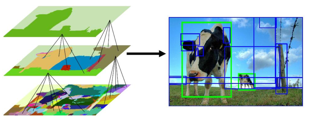
딥러닝에서 사용되던 object detection의 최초는 알고리즘이다. 우선 물체가 있을 만한 곳을 알고리즘을 통해(Region Proposal) 찾아낸 뒤 해당 물체를 CNN을 통해 분류했다(Region Classification).
- Rol(관심 영역) = Selective serch
- object or No object = objectness score
- Bounding box prediction (Bbox regression)
- Class prediction of each box (각 박스 별로 CLASS 예측)
- Non-maximum suppression(NMS) (가장 확률이 높은 박스를 추출)
*NMS?
box와 얼마나 겹치는지, IoU 리스트와 IoU와 같은지 확인(predicted boxes와 ground truth boxes와 비교)
Regions of Insterest(Rol)

Ground Truth와 Object hypotheses를 비교하여 training (positive examples <-> Difficult negativies)
bounding-box Regressor
객체의 bounding Box를 앞에 설명된 네트워크 filter들과의 유사도를 이용하여 거리를 줄여주는 방향으로 학습한다.
- Fram data
#load the image and preprocess it
image = load_img(imagePath, target_size(224,224))
image = imag_to_array(image)

data.append(image)
targets.append((startX, startY, endX, endY))
filenames.append(filename)
...
split = train_test_split(data, targets, filenames, test_size = 0.10, random_state = 42)

(trainImages, testImages) = splist[:2]
(trainTargets, testTargets) = splist[2:4]
(trainFilenames, testFilenames) = splist[4:]
# flatten the max-pooling output of VGG
flatten = vgg.output
flatten = Flatten()(flatten)

#onstruct a fully-connected layer header to output the predicted
#bounding box coordinates
bboxHead = Dense(128, activation = "relu")(flatten)
bboxHead = Dense(64, activation = "relu")(bboxHead)
bboxHead = Dense(32, activation = "relu")(bboxHead)
# 4 : x1, x2, y1, y2
bboxHead = Dense(4, activation = "sigmoid")(bboxHead)

# construct the model we will fine-tune for bounding box regression
model = Model(inputs = vgg.input, ouputs = bboxHead)
opt = Adam(lr = config.INIT_LR)
model.compile(loss = "mse", optimizer = opt)
print(model.summary())

# train the network for bounding box regression 회귀식으로 계산한다.
H = model.fit(
	trainImages, trainTargets,
    validation_data = (testiMages, testTargets),
    batch_size = config.BATCH_SIZE,
    epochs = config.NUM_EPOCHS,
    verbose = 1)

model = load_model(config.MODEL_PATH)

preds = model.predic(image)[0](startX, startY, endX, endY) = preds
Faster R-CNN
- RPN (region proposal network attention network)
ROI 알고리즘으로 Bbox를 찾는 것과 다르게 region proposal가 신경망에 포함됨. 객체의 여부(attention) 확인 - RPN output = (objectness score_객체여부, Bbox)
- Model = VGG16 / ResNet
Anchor
컨볼루션 연산 중 anchor 주변에(sliding window) anchor box를 만들어 regression과 calssification을 수행하며 전체 클래스 결과가 아니라 물체의 여부만 출력한다.
process
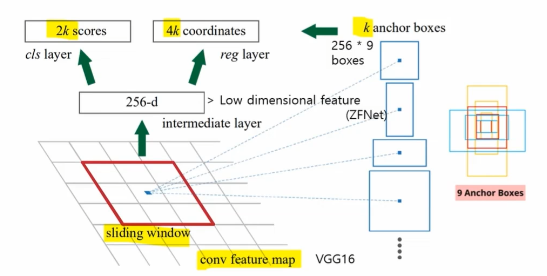
1️⃣ Conv 3x3, 512 channel
2️⃣ Conv 1x1, for background decision (2k scores_cls layer)
3️⃣ Conv 1x1, for Bbox regression (4k coordinates_reg layer)
loss function for taining RPN
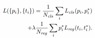
Lcls = objectness (2 classes)
p = predicted object probability
p* = ground-truth ( 1 <- ioU > 0.7, -1 <- ioU < 0.3)
class와 regression의 balancing을 위해 λ를 곱해줌(경험치)
| R-CNN | Fast R-CNN | Faster R-CNN | |
|---|---|---|---|
| 이미지당 시간 | 50s | 2s | 0.2s |
| 속도 | 1x | 25x | 250x |
*그럼에도 불구하고 yolo보다 속도가 낮음
SSD (Single Shot Detector)
- region proposal 신경망을 별도로 통과하니 속도가 떨어지므로 main stream에 ROI에 곧바로 통과하는 방식
- 기존 네트워크(VGG16) 사용
- 격자를 나누어 객체의 크기와 상관없이 찾을 수 있게 설정
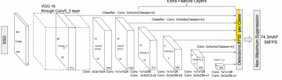
- INPUT = 300X300 이미지
- Conv5_3 layer VGG-16, TOP을 제외한 나머지를 38X38 512층 Conv4_3과 연결
- 여러가지 격자의 GRID를 만듦 (1x1 FC6 Conv6, 1x1 FC7 Conv7,1x1 FC6_2 Conv6_2, 1x1 FC9_2 Conv9_2, 1x1 FC10_2 Conv10_2) 하나하나가 특징 벡터라 생각해도 됨.
- 곧바로 detection하는 layer에 넣음 (Bbox와 class를 정의하는 loss 함수를 이용.)
N = matched boxes number
l = predicted box,
g = ground truth box
이렇듯 같이 loss함수를 정의해서 weight vector를 학습시킴.
achor box 별로 이 형식이 적용 되는데 7x7 형식으로 loss함수로 결합이 되어 계산이 됨.
Yolo ver.1
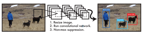
- Resize image (이미지 -> objection)
- Run convolutional network (컨볼루션 네트워크를 이용하여 oneshot에 detection)
- Non-max suppression (class확률이 높은 것 기준으로 sorting)
A single neural network predicts bounding boxes and class probabilities directly from
full images in one evaluation. Since the whole detection
pipeline is a single network(기존: roi층을 별도로 두었기에 속도가 느렸음), it can be optimized end-to-end
directly on detection performance.
Our base
YOLO model processes images in real-time at 45 frames
per second.(SSD)
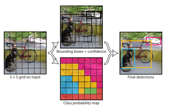
process
- Our system divides the input image into an S × S grid.
- S X S만큼 GRID를 나누고 각 격자마다 bounding box로 dectection 수행
- Each grid cell predicts B bounding boxes and confidence
scores for those boxes.
- confidence
scores(확신률) : grond truth가 되는 어떤 class의 bounding box에 포함이 되는 확률,
- we define confidence as Pr(Object) ∗ IOUtruth
pred .
- 오브젝트가 포함된 비율 x IOU , bounding box가 ground truth에 없으면 계산하지 않음.
- Each bounding box consists of 5 predictions: x, y, w, h,
and confidence.
- object miss
- The (x, y) coordinates represent the center
of the box
- box의 center를 반영
- Each grid cell also predicts C conditional class probabilities, Pr(Classi
|Object).
- class를 prediction
*격자가 7x7로 나눠져 있음.
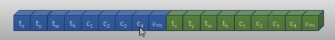
- S × S × (B ∗ 5 + C) tensor
- 격자 x (bounding box*5 + class 개수)
- Our final layer predicts both class probabilities and
bounding box coordinates.
- class에 대한 확률과 bounding box의 좌표
- We normalize the bounding box
width and height by the image width and height so that they
fall between 0 and 1.
- normalize the bounding box
- We parametrize the bounding box x
and y coordinates to be offsets of a particular grid
- bounding box의 x,y 좌표는 상대적인 offset으로 표현
- leaky rectified linear activation
- relu 활성화 함수 사용
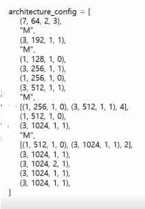
network
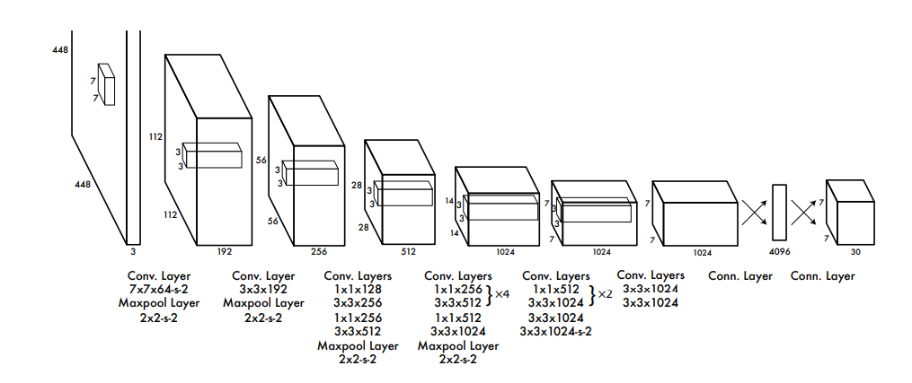
CNNBlock(3, 64, kernel_size = 7, strides = 2, padding = 3)
MaxPool2d(kernel_size = (2,2), stride = (2,2))
해당 코드를 모듈화 시켜서 다음과 같이 표현
class CNNBlock(*nn.Module)
	def __init__(self, in_channels, out_channels, **kwargs):
		super(CNNBlock, self)__init__()
        self.conv = nn.Conv2d(in_channels,out_channels, bias = False, **kwargs)
        self.batchnorm = nn.BatchNorm2d(out_channels)
        self.leakyrelu = nn.leakyReLU(0.1)
   def forward(self, x):
		return self.leakyrelu(self.batchnorm(self.conv(x))
dataset
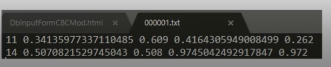
- class와 정규화된 좌표
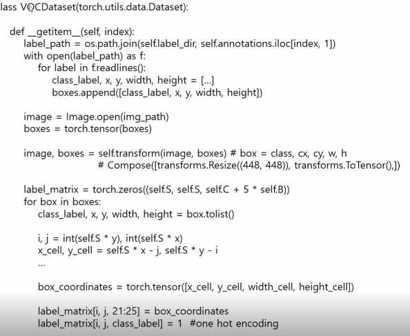
- data = Get_item(index) // epoch마다
- 정답지에 대한 형식을 격자화 시켜서 넣어주어야 함.
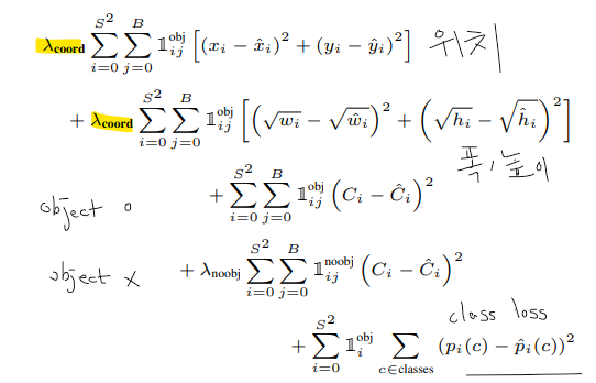
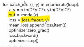
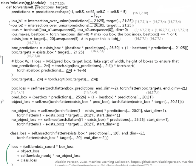
loss function
limit
- yolo ver.1은 작은 객체/겹쳐진 객체는 detection을 잘 수행하지 못함.
