[논문리뷰] Deep Unsupervised Learning using Nonequilibrium Thermodynamics (DPM, 2015)

0. Abstract

• "Diffusion Model"을 최초로 제안한 논문
• non-equilibrium statistical physics에 착안함

1. Introduction

tractability & flexibility tradeoff

• tradeoff in probabilistic models
• models that are tractable
  • e.g. Gaussian or Laplace
  • can be analytically evaluated and easily fit to data
  • 데이터셋이 너무 방대하면 모델링하는데 무리가 있음
• models that are flexible
  • can be molded to fit structure in arbitrary data
  • we can define models in terms of any (non-negative) function $\phi (\mathrm{x})$ yielding the flexible distribution $p(\mathrm{x})=\frac{\phi (\mathrm{x})}{Z}$
  • normalization constant $Z$의 계산이 intractable하기 때문에 flexible model을 train/evaluate/inference 하려면 아주 많은 Monte Carlo process가 필요함

1.1. Diffusion probabilistic models (DPM)

• present DPM that allows
  1. extreme flexibility in model structure
  2. exact sampling
  3. easy multiplication with other distributions (to compute posterior)
  4. can cheaply evaluate log-likelihood and probability of individual states

2. Algorithm

2.0. Overview

• 먼저 target (data) distribution --> simple known (Gaussian) distribution으로 보내는 forward diffusion process를 정의
• finite-time reversal of diffusion process를 학습
• also derive entropy bounds

2.1. Forward Trajectory

• data dist. $q(\mathrm{x}^{(0)})$ --> tractable dist. $\pi (\mathrm{y})$ by repeated Markov diffusion kernel $T_{\pi}(\mathrm{y}|\mathrm{y}';\beta)$ for $\pi (\mathrm{y})$ where $\beta$ is the diffusion rate
  $\begin{aligned} \pi (\mathrm{y})=\int d\mathrm{y}'\ T_{\pi}(\mathrm{y}|\mathrm{y}';\beta)\ \pi(\mathrm{y}') \end{aligned}$
  $\begin{aligned} \mathrm{Forward \ Diffusion\ kernel:}\ q(\mathrm{x}^{(t)}|\mathrm{x}^{(t-1)})&=T_{\pi}(\mathrm{x}^{(t)}|\mathrm{x}^{(t-1)};\beta_{t}) \\ &= \mathcal{N}(\mathrm{x}^{(t)};\mathrm{x}^{(t-1)}\sqrt{1-\beta_{t}},\ \mathrm{I}\beta_{t}) \mathrm{\ if\ Gaussian} \end{aligned}$
  $\begin{aligned} \mathrm{Forward \ Trajectory:}\ q(\mathrm{x^{(0...T)}})=q(\mathrm{x}^{(0)})\ \Pi_{t=1}^{T}\ q(\mathrm{x}^{(t)}|\mathrm{x}^{(t-1)}) \end{aligned}$
• $q(\mathrm{x}^{(t)}|\mathrm{x}^{(t-1)})$은 Gaussian -> Gaussian(with identity coveariance) 또는 Binomial -> Binomial(independent)으로 보내는 kernel이다

2.2. Reverse Trajectory

• Gaussian/Binomial이고 continuous한 diffusion에 대해 (+ 충분히 작은 step size $\beta$), reverse process는 forward process와 같은 functional form을 가진다 (Feller, 1949)
• 학습할 때는
  • Gaussian : 각 kernel의 mean $\mathrm{f}_{\mu}\ (\mathrm{x}^{(t)},t)$과 covariance $\mathrm{f}_{\Sigma}\ (\mathrm{x}^{(t)},t)$
  • Binomial : 각 kernel의 bit flip probability $\mathrm{f}_{b}\ (\mathrm{x}^{(t)},t)$
  • 를 학습한다

2.3. Model Probability

• 데이터에 대한 generative model의 확률은
  $p(\mathrm{x}(0))=∫d\mathrm{x}^{(1⋯T)}p(\mathrm{x}^{(0⋯T)})$
• 원래 이 계산은 intractable하지만, 아래와 같이 바꿔 쓸 수 있다
  - based on annealed importance sampling & Jarzynski equality
  - instead evaluate the relative probability of forward & reverse trajectories, averaged over forward trajectories
  $\begin{aligned} p(\mathrm{x}^{(0)})&=∫d\mathrm{x}^{(1⋯T)} p(\mathrm{x}^{(0⋯T)}) \frac{q(\mathrm{x}^{(1⋯T)}|\mathrm{x}^{(0)})} {q(\mathrm{x}^{(1⋯T)}|\mathrm{x}^{(0)})}\\ &=∫d\mathrm{x}^{(1⋯T)} q(\mathrm{x}^{(1⋯T)}|\mathrm{x}^{(0)}) \frac{p(\mathrm{x}^{(0⋯T)})} {q(\mathrm{x}^{(1⋯T)}|\mathrm{x}^{(0)})}\\ &=∫d\mathrm{x}^{(1⋯T)} q(\mathrm{x}^{(1⋯T)}|\mathrm{x}^{(0)})\ \cdot p(\mathrm{x}^{(T)})∏_{t=1}^{T} \frac{p(\mathrm{x}^{(t-1)}|\mathrm{x}^{(t)})}{q(\mathrm{x}^{(t)}|\mathrm{x}^{(t-1)})} \end{aligned}$
• This can be evaluated rapidly by averaging over samples from the forward trajectory $q(\mathrm{x}^{(1⋯T)}|\mathrm{x}^{(0)})$
• For infinitesimal $\beta$,
  • forward & diffusion kernel이 identical해짐
  • then only a single sample from $q(\mathrm{x}^{(1⋯T)}|\mathrm{x}^{(0)})$ is required to evaluate the above integral

2.4. Training

• Training amounts to maximize the model log likelihood
  $\begin{aligned} L&=\int d\mathrm{x}^{(0)} q(\mathrm{x}^{(0)})\ \mathrm{log}\ p(\mathrm{x}^{(0)})\\ &= \int d\mathrm{x}^{(0)} q(\mathrm{x}^{(0)})\ \cdot\\ &\mathrm{log}\left[∫d\mathrm{x}^{(1⋯T)} q(\mathrm{x}^{(1⋯T)}|\mathrm{x}^{(0)})\ \cdot p(\mathrm{x}^{(T)})∏_{t=1}^{T} \frac{p(\mathrm{x}^{(t-1)}|\mathrm{x}^{(t)})}{q(\mathrm{x}^{(t)}|\mathrm{x}^{(t-1)})}\right] \end{aligned}$
• which has a lower bound provided by Jensen's inequality,
  $\begin{aligned} L\geq &\int d\mathrm{x}^{(0...T)} q(\mathrm{x}^{(0...T)})\ \cdot\\ &\mathrm{log}\left[p(\mathrm{x}^{(T)})∏_{t=1}^{T} \frac{p(\mathrm{x}^{(t-1)}|\mathrm{x}^{(t)})}{q(\mathrm{x}^{(t)}|\mathrm{x}^{(t-1)})}\right]=K \end{aligned}$
• Appendix B에 의해 $K$는 anlytical하게 계산 가능한 entropies와 KL divergences로 정리된다
  $\begin{aligned} K&=-\Sigma_{t=1}^{T} \int\ d\mathrm{x}^{(0)}d\mathrm{x}^{(t)}q\ (\mathrm{x}^{(0)},\mathrm{x}^{(t)})\ \cdot D_{KL}(q\ (\mathrm{x}^{(t-1)}|\mathrm{x}^{(t)}, \mathrm{x}^{(0)})\ ||\ p\ (\mathrm{x}^{(t-1)}|\mathrm{x}^{(t)}))\\ &+ H_{q}(\mathrm{X}^{(T)}|\mathrm{X}^{(0)}) - H_{q}(\mathrm{X}^{(1)}|\mathrm{X}^{(0)}) - H_{p}(\mathrm{X}^{(T)}) \end{aligned}$
• $\beta$가 충분히 작아서 forward process $\approx$ reverse process가 되면 $L = K$
• training은 $K$를 maximize하는 reverse Markov transitions 를 찾는 방향으로 진행됨
  - $\hat{p}(\mathrm{x}^{(t-1)}|\mathrm{x}^{(t)})=\ \underset{p(\mathrm{x}^{(t-1)}|\mathrm{x}^{(t)})}{\mathrm{argmax}}\ K$
• probability distribution estimation은 sequence of Gaussians로 이루어진 function을 regression한는 task로 reduced된다

2.4.1. Setting the Diffusion Rate $\beta_{t}$

• beta scheduling은 모델 성능에 큰 영향을 미침
• Gaussian의 경우 $\beta_{2...T}$를 $K$의 gradient ascent에 따라 달라지게 설정했음
  - 단, overfitting을 막기 위해 $\beta_{1}$은 small constant로 고정
• Binomial의 경우 $\beta_{t}=(T-t+1)^{-1}$로 freeze
• 후속 연구들에 따르면 Gaussian도 fixed schedule로 고정하는 게 낫다고 함

2.5. Multiplying Distributions, and Computing Posteriors

2.5.1. Modified Marginal Distributions

2.5.2. Modified Diffusion Steps

2.5.3. Applying $r(\mathrm{x}^{(t)})$

2.5.4. Choosing $r(\mathrm{x}^{(t)})$

2.6. Entropy of Reverse Process

3. Experiments

3.1. Toy Problems

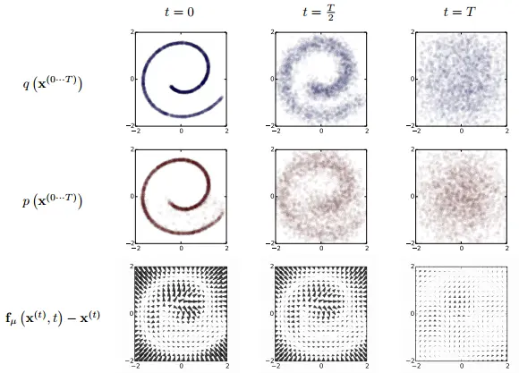
• 3.1.1. Swiss Roll

  • 2D swiss roll dist. 학습

  • RBF network로 mean $\mathrm{f}_{\mu}\ (\mathrm{x}^{(t)},t)$과 covariance $\mathrm{f}_{\Sigma}\ (\mathrm{x}^{(t)},t)$ 생성하게 함

  • 

  • 그림에서 세 번째 행은 drift term에 해당함

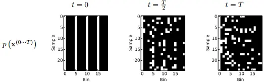
• 3.1.2. Binary Heartbeat Distribution

  • length 20짜리 simple binary sequences로 학습
    • 1 occurs every 5th time bin (나머지는 0)
  • MLP로 Bernoulli rates $\mathrm{f}_{b}\ (\mathrm{x}^{(t)},t)$ 생성하게 함
  • 

3.2. Images

• multi-scale convolutional architectures used
• MNIST, CIFAR-10, Dead Leaf Images, Bark Texture Images
• generation & inpainting task

Appendix

A. Conditional Entropy Bounds Derivation

B. Log Likelihood Lower Bound

• initial lower bound of the log likelihood

  $\begin{aligned} K=\int d\mathrm{x}^{(0...T)} q(\mathrm{x}^{(0...T)})\ \mathrm{log}[p(\mathrm{x}^{(T)})∏_{t=1}^{T} \frac{p(\mathrm{x}^{(t-1)}|\mathrm{x}^{(t)})}{q(\mathrm{x}^{(t)}|\mathrm{x}^{(t-1)})}] \end{aligned}$

• B.1. Entropy of $p(\mathrm{X}^{(T)})$
  

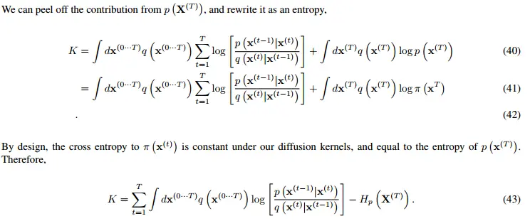
• B.2. Remove the edge effect at $t=0$
  

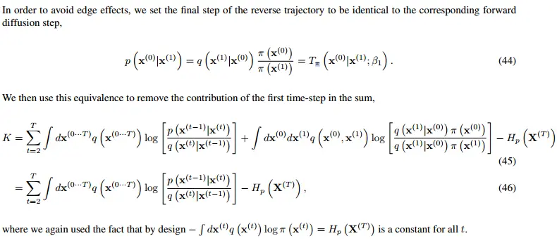
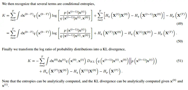
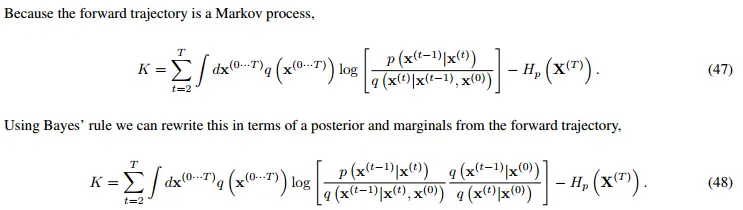
• B.3. Rewrite in terms of posterior $q(\mathrm{x}^{(t-1)}|\mathrm{x}^{(0)})$
  

• B.4. Rewrite in terms of KL divergences and entropies
  

C. Perturbed Gaussian Transition