
01. 로지스틱 회귀(Logistic Regression)
- 이진 분류 문제를 풀기 위한 대표적인 알고리즘으로 로지스틱 회귀가 있음.
- 이진 분류 문제 예시
- 시험 결과가 합격인지 불합격인지
- 스팸메일인지 아닌지
- 이진 분류 문제 예시
- 이름은 '회귀'지만 실제로 분류(Classifiction) 작업에 사용됨.
1. 이진 분류
- 학생들의 시험 성적에 따라서 합격, 불합격이 기재된 데이터가 있다고 가정
- 시험성적이 라면 합불 결과는
- 시험의 커트라인은 모르지만 특정 점수를 얻었을때, 합격/불합격 여부를 판정하는 모델을 만들고자 함.
| score() | result() |
|---|---|
| 45 | 불합격 |
| 50 | 불합격 |
| 55 | 불합격 |
| 60 | 합격 |
| 65 | 합격 |
| 70 | 합격 |
- 합격(1) 또는 불합격(0)으로 나뉘므로 직선을 사용할 경우 분류 작업이 잘 동작하지 않음.
- S자 모양의 그래프를 만들 수 있는 어떤 특정 함수 를 사용해야 함.
- 의 가설을 사용
- S자 모양의 그래프를 그릴 수 있는 함수는 시그모이드 함수
2. 시그모이드 함수(Sigmoid function)
- 시그모이드 함수의 방정식은 아래와 같음.
- 선형회귀와 마찬가지로 최적의 기울기()와 y절편()를 찾는 것이 목표
- 시그모이드 함수에서 와 가 함수의 그래프에 어떤 영향을 줄까?
import numpy as np
import matplotlib.pyplot as plt
def sigmoid(x):
# 시그모이드 함수 정의
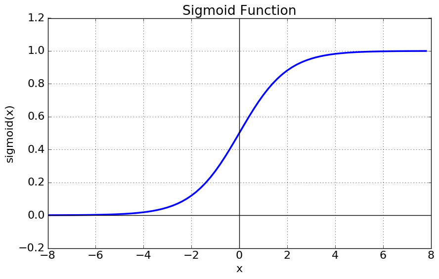
return 1/(1+np.exp(-x))1. W가 1이고 b가 0인 그래프
x=np.arange(-5.0,5.0,0.1)
y=sigmoid(x)

plt.plot(x,y,'g')
plt.plot([0,0],[1.0,0.0],':') # 가운데 점선 추가
plt.title('Sigmoid Function')
plt.show()- 위의 그래프를 통해 시그모이드 함수의 출력값 범위는 (0,1)임을 알 수 있음.
- 가 0일때 0.5의 값을 가짐
- 가 매우 커지면 1에 수렴하고 매우 작아지면 0에 수렴함.
2. W값의 변화에 따른 경사도의 변화
x=np.arange(-5.0,5.0,0.1)
y1=sigmoid(0.5*x)
y2=sigmoid(x)
y3=sigmoid(2*x)

plt.plot(x,y1,'r',linestyle='--') #W의 값이 0.5일때
plt.plot(x,y2,'g') #W의 값이 1일때
plt.plot(x,y3,'b',linestyle='--') #W의 값이 2일때
plt.plot([0,0],[1.0,0.0],':') #가운데 점선 추가
plt.title('Sigmoid Function')
plt.show()- 의 값에 따라 그래프의 경사도가 변하는 것을 볼 수 있음.
- 선현 회귀에서 가중지 는 직선의 기울기를 의미, 시그모이드는 그래프의 경사도를 결정
- 의 값이 커지면 경사가 커지고 의 값이 작아지면 경사가 작아짐.
3. b값의 변화에 따른 좌, 우 이동
x=np.arange(-5.0,5.0,0.1)
y1=sigmoid(x+0.5)
y2=sigmoid(x+1)
y3=sigmoid(x+1.5)

plt.plot(x,y1,'r',linestyle='--') #W의 값이 0.5일때
plt.plot(x,y2,'g') #W의 값이 1일때
plt.plot(x,y3,'b',linestyle='--') #W의 값이 2일때
plt.plot([0,0],[1.0,0.0],':') #가운데 점선 추가
plt.title('Sigmoid Function')
plt.show()- 의 값에 따라서 그래프가 좌, 우로 이동하는 것을 보여줌.
4. 시그모이드 함수를 이용한 분류
- 시그모이드 함수는 입력값이 한없이 커지면 1에 수렴하고, 입력값이 한없이 0에 수렴함.
- 임계값을 0.5라고 정했을때, 출력값이 0.5 이상이면 1(True), 0.5이하이면 0(False)으로 판단.
- 해당 레이블에 속할 확률이 50%가 넘으면 해당 레이블로 판단하고, 해당 레이블에 속할 확률이 50%보다 낮으면 아니라고 판단.
3. 비용함수(Cost Function)
- 로지스틱 회귀의 가설:
- 최적의 와 를 찾을 수 있는 비용함수를 정의해보자.
- 선형회귀에서 사용했던 MSE의 수식
$cost(W,b)=\frac{1}{n} \sum_{i=1}^{n} [y^{(i)}-H(x^{(i)}]^2 $ - 를 함수로 치환해서, 비용함수를 미분하면 다음과 같이 심한 비볼록(non-convex) 형태의 그래프가 나옴.

- 전체 함수에 걸쳐 최소값인 글로벌 미니멈이 아닌 특정 구역에서의 최소값인 로컬 미니멈에 도달할 수 있음.
- cost가 최소가 되는 가중치 를 찾는다는 비용함수의 목적에 맞지 않음.
- 시그모이드 함수의 특징는 함수의 출력값이 0과 1사이의 값이라는 점.
- 실제값이 1일때 예측값이 0에 가까워지면 오차가 커져야 하며, 실제값이 0일대, 예측값이 1에 가까워지면 오차가 커져야 함.
- 이를 충족하는 함수는 로그함수

- 실제값이 1일때의 그래프를 주황색, 실제값이 0일때의 그래프를 초록색으로 표현.
- 예시 참고 : 실제값이 1인경우
- 예측값인 의 값이 1이면 오차가 0이므로 당연히 cost는 0이 됨.
- 예측값인 의 값이 0이면 cost는 무한대로 발산
- 예시 참고 : 실제값이 1인경우
$$ if\; y=1 \rightarrow cost(H(x),y) = -log(H(x)) if\; y=0 \rightarrow cost(H(x),y) = -log(1-H(x))$$
-
y의 실제값이 1일때 그래프를 사용하고 의 실제값이 0일때, 그래프를 사용해야함.
$$ cost(W)=-\frac{1}{n}\sum_{i=1}^{n} [y^{(i)}logH(x^{(i)})+(1-y^{(i)})log(1-H(x^{(i)})] $$ -
정리하면, 위 비용 함수는 실제값 와 예측값 의 차이가 커지면 cost가 커지고, 실제값 와 예측값 의 차이가 작아지면 cost는 작아짐.
-
위 비용함수에 대해서 경사하강법을 수행하면서 최적의 가중치 를 찾아감.
4. 파이토치로 로지스틱 회귀 구현하기
- 다수의 로부터 를 예측하는 다중 로지스틱 회귀를 구현함.
1. 패키지 선언 및 초기화
import torch
import torch.nn as nn
import torch.nn.functional as F
import torch.optim as optimtorch.manual_seed(1)2. 훈련데이터 선언
x_data=[[1,2],[2,3],[3,1],[4,3],[5,3],[6,2]]
y_data=[[0],[0],[0],[1],[1],[1]]
x_train=torch.FloatTensor(x_data)
y_train=torch.FloatTensor(y_data)

print(x_train.shape)
print(y_train.shape)torch.Size([6, 2])
torch.Size([6, 1])3. W, b 선언
W = torch.zeros((2,1),requires_grad=True)
b = torch.zeros(1,requires_grad=True)
4. 가설 설정
# 시그모이드 정의 대로 식 설정
hypothesis = 1 / (1 + torch.exp(-(x_train.matmul(W)+b)))
# torch를 통해 구현
hypothesis = torch.sigmoid(x_train.matmul(W)+b)

print(hypothesis)
print(y_train)
#hypothesis
tensor([[0.5000],
[0.5000],
[0.5000],
[0.5000],
[0.5000],
[0.5000]], grad_fn=<SigmoidBackward0>)
# answer
tensor([[0.],
[0.],
[0.],
[1.],
[1.],
[1.]])5. 비용함수 설정
- 오차를 구하는 식
- 하나의 샘플에 대해서 cost 연산
-(y_train[0] * torch.log(hypothesis[0])) + (1-y_train[0]) * torch.log(1-hypothesis[0])- 전체 샘플에 대해서 cost 연산
losses= -(y_train * torch.log(hypothesis) + (1-y_train) * torch.log(1-hypothesis))
cost = losses.mean()

print(losses)
print(cost)tensor([[0.6931],
[0.6931],
[0.6931],
[0.6931],
[0.6931],
[0.6931]], grad_fn=<NegBackward0>)
tensor(0.6931, grad_fn=<MeanBackward0>)torch.nn.functional에서 제공하는 비용함수
# torch.nn.functional as F에서 제공하는 비용함수 binary_cross_entropy(예측값, 실제값)
F.binary_cross_entropy(hypothesis,y_train)
x_data = [[1,2],[2,3],[3,1],[4,3],[5,3],[6,2]]
y_data = [[0],[0],[0],[1],[1],[1]]
x_train = torch.FloatTensor(x_data)
y_train = torch.FloatTensor(y_data)6. 모델 학습
# 모델 초기화
W = torch.zeros((2,1), requires_grad= True)
b = torch.zeros(1, requires_grad=True)

# optimizer 설정
optimizer=optim.SGD([W,b], lr=1)

nb_epochs=1000
for epoch in range(nb_epochs+1):

    # Cost 계산
    hypothesis=torch.sigmoid(x_train.matmul(W)+b)
    cost=-(y_train * torch.log(hypothesis) + (1-y_train)*torch.log(1-hypothesis)).mean()

    optimizer.zero_grad()
    cost.backward()
    optimizer.step()

    if epoch % 100 == 0:
        print('Epoch {:4d}/{} Cost {:.6f}'.format(epoch,nb_epochs,cost.item()))
Epoch 0/1000 Cost 0.693147
Epoch 100/1000 Cost 0.134722
...
Epoch 900/1000 Cost 0.021888
Epoch 1000/1000 Cost 0.0198527. 가중치 출력
print(W)
print(b)tensor([[3.2530],
[1.5179]], requires_grad=True)
tensor([-14.4819], requires_grad=True)