

Prophet은 시계열 데이터를 예측하기 위한 강력한 오픈 소스 예측 라이브러리입니다. 이를 통해 비전문가들도 상대적으로 쉽게 사용할 수 있도록 설계되어 있습니다. Prophet은 주기적인 패턴이나 휴일 효과와 같은 시계열 데이터의 특성을 자동으로 학습하여 예측을 수행합니다. Prophet을 사용하면 비전문가도 비교적 손쉽게 효과적인 시계열 예측 모델을 구축할 수 있습니다.
시계열분석?
시계열 분석은 시간의 경과에 따라 발생한 데이터를 분석하고 모델링하는 통계적인 방법입니다. 주로 시계열 데이터는 일정 시간 간격으로 관측된 데이터의 순서적인 열을 나타냅니다.
설치하기
pip install prophet
pip install pandas_datareader
준비하기
from pandas_datareader import data
from prophet import Prophet
import matplotlib.pyplot as plt
import numpy as np
import pandas as pd
%matplotlib inline
from matplotlib import rc
rc('font', family='Arial Unicode MS')
# 간단한 데이터 재료 준비
time = np.linspace(0, 1, 365*2)
result = np.sin(2*np.pi*12*time)
ds = pd.date_range('2017-01-01', periods=365*2, freq = 'D')
df = pd.DataFrame({'ds':ds, 'y':result})
df.head()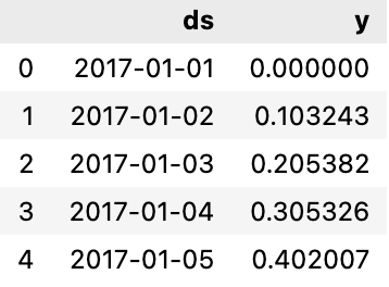
시계열 분석
m = Prophet(yearly_seasonality=True, daily_seasonality=True)
m.fit(df);

future = m.make_future_dataframe(periods=30)
forecast = m.predict(future)

m.plot(forecast)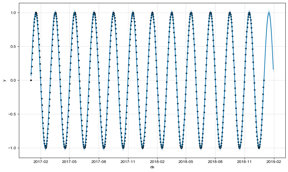
점이 찍힌 구간이 기존의 데이터이고 오른쪽 점이 없는 구간은 시계열 분석을 통해 예측한 값입니다.
노이즈 추가
time = np.linspace(0, 1, 365*2)
result = np.sin(2*np.pi*12*time) + time + np.random.randn(365*2)/4

ds = pd.date_range('2017-01-01', periods=365*2, freq = 'D')
df = pd.DataFrame({'ds':ds, 'y':result})

df['y'].plot(figsize=(10,6))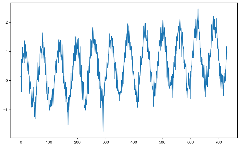
m = Prophet(yearly_seasonality=True, daily_seasonality=True)
m.fit(df)
future = m.make_future_dataframe(periods=30)
forecast = m.predict(future)
m.plot(forecast);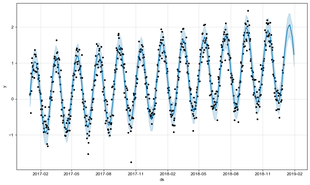
웹데이터 시계열 분석해보기
pinkwink_web = pd.read_csv(
    "data/05_PinkWink_Web_Traffic.csv",
    encoding="utf-8",
    thousands=",",
    names=["date","hit"],
    index_col = 0,
)
pinkwink_web = pinkwink_web[pinkwink_web["hit"].notnull()]pinkwink_web["hit"].plot(figsize=(12,4), grid = True);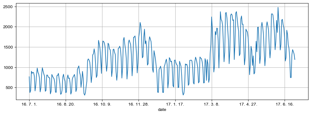
df = pd.DataFrame({"ds": pinkwink_web.index, "y":pinkwink_web["hit"]})
df.reset_index(inplace=True)
df["ds"] = pd.to_datetime(df["ds"], format="%y. %m. %d.")
del df["date"]
df.head()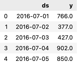
m = Prophet(yearly_seasonality=True, daily_seasonality=True)
m.fit(df);
future = m.make_future_dataframe(periods=60)
forecast = m.predict(future)
forecast[["ds", "yhat", "yhat_lower", "yhat_upper"]].tail()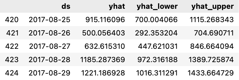
forecast.info()<class 'pandas.core.frame.DataFrame'> RangeIndex: 425 entries, 0 to 424 Data columns (total 22 columns): # Column Non-Null Count Dtype --- ------ -------------- ----- 0 ds 425 non-null datetime64[ns] 1 trend 425 non-null float64 2 yhat_lower 425 non-null float64 3 yhat_upper 425 non-null float64 4 trend_lower 425 non-null float64 5 trend_upper 425 non-null float64 6 additive_terms 425 non-null float64 7 additive_terms_lower 425 non-null float64 8 additive_terms_upper 425 non-null float64 9 daily 425 non-null float64 10 daily_lower 425 non-null float64 11 daily_upper 425 non-null float64 12 weekly 425 non-null float64 13 weekly_lower 425 non-null float64 14 weekly_upper 425 non-null float64 15 yearly 425 non-null float64 16 yearly_lower 425 non-null float64 17 yearly_upper 425 non-null float64 18 multiplicative_terms 425 non-null float64 19 multiplicative_terms_lower 425 non-null float64 20 multiplicative_terms_upper 425 non-null float64 21 yhat 425 non-null float64 dtypes: datetime64[ns](1), float64(21) memory usage: 73.2 KB
용어정리
- ds : 날짜 및 시간 정보를 나타내는 열입니다.
- trend : 전반적인 추세를 나타내는 열로, 시간에 따른 데이터의 일반적인 증감 추이를 나타냅니다.
- yhat_lower : 예측 값의 최소 하한선(lower bound)을 나타내는 열입니다.
- yhat_upper : 예측 값의 최대 상한선(upper bound)을 나타내는 열입니다.
- trend_lower, trend_upper : 추세의 최소 및 최대 경계를 나타내는 열입니다.
- additive_terms : 일일, 주간, 연간 등의 추가적인 성분을 나타내는 열입니다.
- additive_terms_lower, additive_terms_upper : 추가적인 성분의 최소 및 최대 경계를 나타내는 열입니다.
- daily, daily_lower, daily_upper: 일일 성분에 대한 값과 그 최소 및 최대 경계를 나타내는 열입니다.
- weekly, weekly_lower, weekly_upper: 주간 성분에 대한 값과 그 최소 및 최대 경계를 나타내는 열입니다.
- yearly, yearly_lower, yearly_upper: 연간 성분에 대한 값과 그 최소 및 최대 경계를 나타내는 열입니다.
- multiplicative_terms, multiplicative_terms_lower, multiplicative_terms_upper : 곱셈 항(multiplicative term)에 대한 값과 그 최소 및 최대 경계를 나타내는 열입니다.
- yhat : 전체 예측 최종값입니다.
m.plot_components(forecast);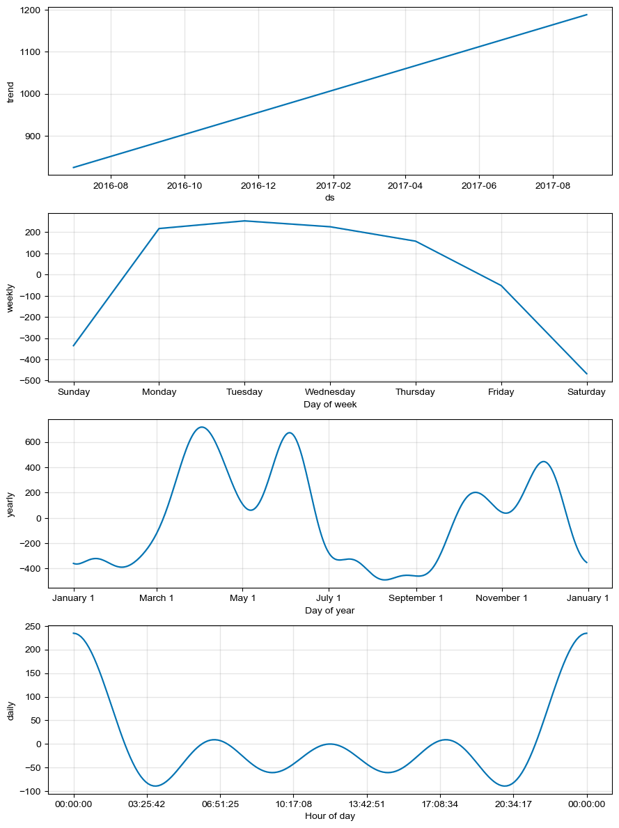
m.plot(forecast);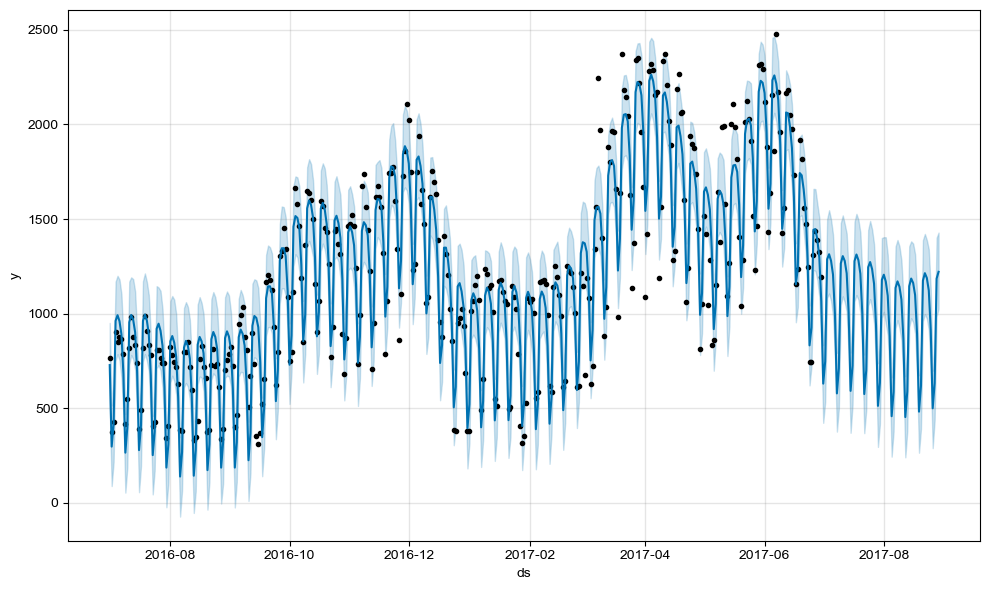
plot_components()를 통해 날짜별, 시간대별 분석이 가능합니다.

낭만젊음사랑