PyTorch 기본

c0natus·2022년 1월 24일

PyTorch

목록 보기

1/4

1. PyTorch vs TensorFlow

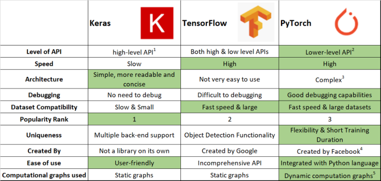
많은 딥러닝 프레임워크가 있지만, 리더는 PyTorch와 TensorFlow이다.

Keras는 wrapper로, interface는 사용자가 사용하기 쉽지만 내부는 TensorFlow나 PyTorch로 구현되어 있다.
Keras의 속도는 완전 느리지 않다. 창시자가 구글에 있다보니 TensorFlow와 결합하게 되어 유지/보수가 되기 때문이다.
인기도(popularity)는 분야에 따라 달라진다.
PyTorch와 TensorFlow의 가장 큰 차이는 마지막 부분인 Computational graphs used이다.

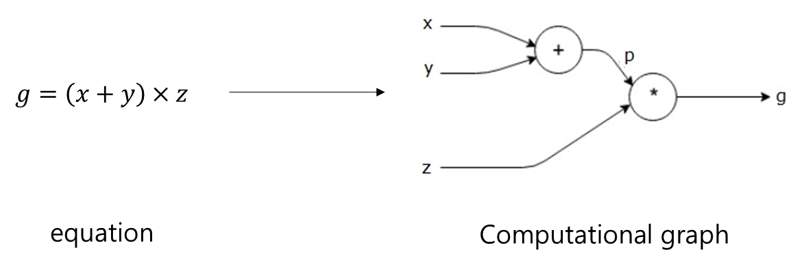
Computational graphs는 연산의 과정을 그래프로 표현하는 것이다. 두 프레임워크는 역전파 과정에서 자동미분을 할 때, 연산과정을 그래프로 그리는 시점에서 차이가 발생한다.

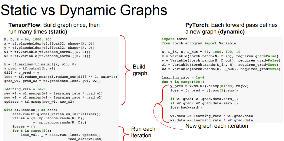
1.1. Static vs Dynamic Graphs

TensorFlow는 Define and Run 방법으로 그래프를 위와 같이 먼저 코드로 정의한 후, 실행 시점에 데이터를 feed한다.
PyTorch는 Define by Run 방법(DCG: Dynamic Computational Graph)으로 실행을 하면서 그래프를 생성하는 방식이다.
DCG 방식이 중간에 미분 값을 확인할 수 있어, 디버깅할 때 더 편하다.
TensorFlow는 production, scalability, Multi GPU 등 에서 강점을 가진다.
PyTorch는 논문 구현, 아이디어 구현, 사용의 편리성 등에서 강점을 가진다.

1.2. PyTorch 특징

PyTorch의 핵심 부분은 Numpy, AutoGrad(자동미분), Function이다.

Numpy 구조를 가지는 Tensor 객체로 array를 표현한다.

자동미분을 지원하여 DL 연산을 지원한다.

다양한 형태의 DL을 지원하는 함수와 모델을 지원한다.

자동미분이 딥러닝 프레임워크의 핵심부분이다.
Dataset, Multi-GPU 등의 다양한 함수와 모델을 지원한다.
이런 특징들로, PyTorch는 비교적 쉽게 사용할 수 있다는 장점을 가진다.

2. PyTorch 기초 문법: Class Tensor

PyTorch는 Numpy 기반으로 만들었기 때문에 문법은 자동미분을 제외하고 Numpy와 유사하다.
다차원 Arrays를 표현하는 PyTorch 클래스이다.
시살상 numpy의 ndarray와 동일하고, TensorFlow의 Tensor와도 동일하다.
Tensor를 생성하는 함수도 거의 동일하다.

import numpy as np

n_array = np.arange(10).reshape(2,5)
print(n_array)
print("ndim :", n_array.ndim, "shape :", n_array.shape)

# 결과
#
# [[0 1 2 3 4]
#  [5 6 7 8 9]]
# ndim : 2 shape : (2, 5)

import torch

t_array = torch.FloatTensor(n_array)
print(t_array)
print("ndim :", t_array.ndim, "shape :", t_array.shape)

# 결과
#
# tensor([[0., 1., 2., 3., 4.],
#         [5., 6., 7., 8., 9.]])
# ndim : 2 shape : torch.Size([2, 5])

Tensor 생성에 list나 ndarray를 사용할 수 있다.

# data to tensor
data = [[3, 5],[10, 5],]
x_data = torch.tensor(data)

# ndarray to tensor
nd_array_ex = np.array(data)
tensor_array = torch.from_numpy(nd_array_ex)

DL에서 Tensor를 생성하는 일을 별로 없다.

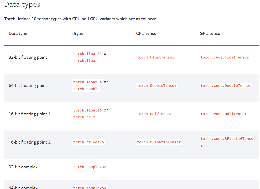
2.1. Tensor data Type

Tensor의 data type은 numpy와 유사하지만, GPU tensor를 추가적으로 가진다.
GPU tensor는 GPU를 쓸 수 있게 해준다.
자세한 내용은 아래 reference를 참고하자.

2.2. Tensor operations

기본적으로 numpy의 대부분의 사용법이 PyTorch에 적용된다.

import numpy as np
import torch

data = [[3, 5, 20],[10, 5, 50], [1, 5, 10]]
x_data = torch.tensor(data)

print(x_data[1:])

# 결과
#
# tensor([[10,  5, 50],
#         [ 1,  5, 10]])

print(x_data[:2, 1:])

# 결과
#
# tensor([[ 5, 20],
#         [ 5, 50]])

print(x_data.flatten())

# 결과
#
# tensor([ 3,  5, 20, 10,  5, 50,  1,  5, 10])

print(torch.ones_like(x_data))

# 결과
# 
# tensor([[1, 1, 1],
#         [1, 1, 1],
#         [1, 1, 1]])

print(x_data.numpy())

# 결과
#
# array([[ 3,  5, 20],
#       [10,  5, 50],
#       [ 1,  5, 10]])


print(x_data.shape)
print(x_data.dtype)

# 결과
#
# torch.Size([3, 3])
# torch.int64

PyTorch의 tensor는 GPU에 올려서 사용가능하다.

print(x_data.device)

# 결과
#
# device(type='cpu')

if torch.cuda.is_available():
    x_data_cuda = x_data.to('cuda')
print(x_data_cuda.device)

# 결과
#
# device(type='cuda', index=0)

덧셈, 슬라이스, 뺄셈 등은 numpy와 동일하지만, 행렬곱셈 연산에서 차이가 난다.
행렬곱셈 연산의 함수는 dot이 아닌 mm을 사용한다.
PyTorch에서는 내적의 연산(dot)과 행렬곱셈 연산(mm)을 구분한다.
matmul은 mm과 동일한 기능을 하지만, matmul은 mm과 다르게 broadcasting을 지원하여 처리한다.

a = torch.rand(5, 2, 3)
b = torch.rand(5)
a.mm(b)

# 결과
#
# error

# 5는 batch size, 2 x 3 행렬과 3 x 1 행렬의 곱셈
# 따라서 결과는 5 x 2 x 1 행렬이 된다.
a = torch.rand(5, 2, 3)
b = torch.rand(3)
a.matmul(b)

# 결과
#
# tensor([[0.2700, 0.3807],
#         [0.5270, 0.4182],
#         [0.3577, 0.4374],
#         [0.1954, 0.2551],
#         [0.2503, 0.2015]])

# 아래의 결과는 matmul 결과와 같다.
# unsqueeze, saqueeze는 바로 아래에서 알아보자.
a[0].mm(torch.unsqueeze(b, 1)).squeeze()
a[1].mm(torch.unsqueeze(b, 1)).squeeze()
a[2].mm(torch.unsqueeze(b, 1)).squeeze()
a[3].mm(torch.unsqueeze(b, 1)).squeeze()
a[4].mm(torch.unsqueeze(b, 1)).squeeze()

matmul은 헷갈릴 수 있기 때문에, mm 쓰는 것을 권장한다.

2.3. Tensor handling: view, squeeze, unsqueeze

view는 reshape과 동일하게 tensor의 shape을 변환한다.
view와 reshape의 차이는 contiguity 보장이다.
view는 contiguity를 보장하고, reshape은 contiguity를 보장하지 않는다.
view 쓰는 것을 권장한다.

import tensor

# view vs reshape

a = torch.zeros(3, 2)
b = a.view(2, 3)
a.fill_(1)

print(f"a: {a}")
print(f"b: {b}")

# 결과
#
# a: tensor([[1., 1.],
#        [1., 1.],
#        [1., 1.]])
# b: tensor([[1., 1., 1.],
#         [1., 1., 1.]])

a = torch.zeros(3, 2)
b = a.t().reshape(6)
a.fill_(1)

print(f"a: {a}")
print(f"b: {b}")

# 결과
#
# a: tensor([[1., 1.],
#         [1., 1.],
#         [1., 1.]])
# b: tensor([0., 0., 0., 0., 0., 0.])

squeeze는 차원의 개수가 1인 차원을 삭제(압축)하고, unsqueeze는 차원의 개수가 1인 차원을 추가한다.
squeeze와 unsqueeze는 BERT 모델에서 자주 사용된다.

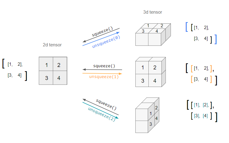
unsqueeze에 지정해주는 것은 dim이다. 이것은 numpy의 axis에 해당 한다.

tensor_ex = torch.rand(size=(2, 1, 2))
print(tensor_ex.shape)
print(tensor_ex)
print(tensor_ex.squeeze())
print(tensor_ex.squeeze().shape)

# 결과
#
# torch.Size([2, 1, 2])
# tensor([[[0.0248, 0.1450]],
# 
#         [[0.1607, 0.0856]]])
#
# torch.Size([2, 2])
# tensor([[0.0248, 0.1450],
#         [0.1607, 0.0856]])

tensor_ex = torch.rand(size=(2, 2))
print(tensor_ex.unsqueeze(0).shape)

# 결과
#
# torch.Size([1, 2, 2])

print(tensor_ex.unsqueeze(1).shape)

# 결과
#
# torch.Size([2, 1, 2])

print(tensor_ex.unsqueeze(2).shape)

# 결과
#
# torch.Size([2, 2, 1])

2.4. Tensor operations for ML/DL formula

nn.functional 모듈을 통해 다양한 수식 변환을 사용할 수 있다.
필요한 것은 찾아서 사용하자.

import torch
import torch.nn.functional as F

tensor = torch.FloatTensor([0.5, 0.7, 0.1])
h_tensor = F.softmax(tensor, dim=0)
h_tensor

# 결과
#
# tensor([0.3458, 0.4224, 0.2318])

import itertools
a = [1, 2, 3]
b = [4, 5]
print(list(itertools.product(a, b)))

# 결과
# [(1, 4), (1, 5), (2, 4), (2, 5), (3, 4), (3, 5)]

tensor_a = torch.tensor(a)
tensor_b = torch.tensor(b)
torch.cartesian_prod(tensor_a, tensor_b)

# 결과
#
# tensor([[1, 4],
#         [1, 5],
#         [2, 4],
#         [2, 5],
#         [3, 4],
#         [3, 5]])

2.5. ✨ AutoGrad(자동 미분)

PyTorch의 핵심은 자동 미분의 지원이다.
requires_grad = True로 설정해야 한다.
'requires_grad = True'는 autograd에 모든 연산(operation)들을 추적해야 한다고 알려준다.

y = w^2

z = 10 \times y + 25

z = 10 \times w^2 + 25

위의 식에서 $w = 2$ 일 때, $\frac{\partial z}{\partial w}$ 의 값을 구해보자.

w = torch.tensor(2.0, requires_grad=True)
y = w**2
z = 10*y + 25
z.backward() # 자동 미분 수행
print(w.grad)

# 결과
#
# tensor(40.)

벡터 편미분

$Q = 3a^3 - b^2$ 에서 $a = <2, 3>, b = <6, 4>$ 일 때, $\frac{\partial Q}{\partial a}$ 의 값을 구해보자.

requires_grad=True를 갖는 2개의 tensor $a, b$ 를 만든다.

$a, b$ 로부터 새로운 텐서 $Q$ 를 만든다.

$a, b$ 가 모두 신경망(NN)의 매개변수이고, $Q$ 가 오차(error)라고 가정한다.

신경망을 학습할 때, 아래와 같이 매개변수들에 대한 오차의 변화도(gradient)를 구해야 한다.

$Q$ 에 대해서 .backward() 를 호출할 때, autograd는 이러한 변화도들을 계산하고 이를 각 텐서( $a, b$ )의 .grad 속성(attribute)에 저장한다.

$Q$ 는 벡터(vector)이므로 Q.backward() 에 gradient 인자(argument)를 명시적으로 전달해야 한다.

gradient 는 $Q$ 와 같은 모양(shape)의 텐서로, $Q$ 자기 자신에 대한 변화도(gradient)를 나타낸다. 즉, $\frac{dQ}{dQ} = 1$ 이다.

이제 변화도는 a.grad 와 b.grad 에 저장된다.

a = torch.tensor([2., 3.], requires_grad=True)
b = torch.tensor([6., 4.], requires_grad=True)
Q = 3*a**3 - b**2

# a벡터 2개의 원소에 대해 미분을 해야하므로
# external_grad를 다음과 같이 잡아줬다.
external_grad = torch.tensor([1., 1.])
Q.backward(gradient=external_grad)

print(a.grad)

# 결과
#
# tensor([36., 81.])

print(b.grad)

# 결과
#
# tensor([-12.,  -8.])

References

c0natus

Done is Better Than Perfect

다음 포스트

PyTorch 기본

PyTorch

1. PyTorch vs TensorFlow

1.1. Static vs Dynamic Graphs

1.2. PyTorch 특징

2. PyTorch 기초 문법: Class Tensor

2.1. Tensor data Type

2.2. Tensor operations

2.3. Tensor handling: view, squeeze, unsqueeze

2.4. Tensor operations for ML/DL formula

2.5. ✨ AutoGrad(자동 미분)

References

PyTorch 구조 - 1

0개의 댓글