책 예제 사용합니다.
책: AICE Associate
책 예제 데이터
Chapter 06 데이터 전처리하기
Section 01 수치형 데이터 정제하기
01) 결측치 파악하기
import random

# 시드 고정
random.seed(420)
np.random.seed(420)

# 랜덤으로 결측치 5,000개 생성
df_na = df.copy()
for i in range(0, 5000):
    df_na.iloc[random.randint(0, 300152), random.randint(0, 10)] = np.nan
(1) 결측치 존재 여부 확인하기
# 데이터 정보 확인
df_na.info()

# <class 'pandas.core.frame.DataFrame'>
# RangeIndex: 300153 entries, 0 to 300152
# Data columns (total 11 columns):
#  #   Column            Non-Null Count   Dtype
# ---  ------            --------------   -----
#  0   airline           299738 non-null  object
#  1   flight            299679 non-null  object
#  2   source_city       299657 non-null  object
#  3   departure_time    299724 non-null  object
#  4   stops             299677 non-null  object
#  5   arrival_time      299743 non-null  object
#  6   destination_city  299732 non-null  object
#  7   class             299670 non-null  object
#  8   duration          299653 non-null  float64
#  9   days_left         299708 non-null  float64
#  10  price             299705 non-null  float64
# dtypes: float64(3), object(8)
# memory usage: 25.2+ MB
(2) 결측치 수 확인하기
# 칼럼 기준으로 결측치 수 확인
df_na.isnull().sum(axis=0)

# airline             417
# flight              471
# source_city         466
# departure_time      455
# stops               439
# arrival_time        462
# destination_city    480
# class               484
# duration            432
# days_left           425
# price               462
# dtype: int64
2) 결측치 처리하기
결측치 처리 방법
1. 결측치가 포함된 레코드 제거
2. 결측치가 포함된 칼럼 제거
3. 결측치 대체
# 데이터 변경에 대비해 원본 데이터 복사
df_na_origin = df_na.copy()
(1) 결측치 삭제
손쉽게 결측치를 처리할 수 있지만, 데이터의 손실이 생겨 원래 데이터 특성을 모두 반영하지 못 하는 문제가 생긴다. 때문에, 결측치 비중이 적을 때 사용하는 것이 좋다.
# 결측치를 하나라도 가지는 행 모두 삭제
df_na = df_na.dropna()
df_na.info()

# <class 'pandas.core.frame.DataFrame'>
# Index: 295190 entries, 0 to 300152
# Data columns (total 11 columns):
#  #   Column            Non-Null Count   Dtype
# ---  ------            --------------   -----
#  0   airline           295190 non-null  object
#  1   flight            295190 non-null  object
#  2   source_city       295190 non-null  object
#  3   departure_time    295190 non-null  object
#  4   stops             295190 non-null  object
#  5   arrival_time      295190 non-null  object
#  6   destination_city  295190 non-null  object
#  7   class             295190 non-null  object
#  8   duration          295190 non-null  float64
#  9   days_left         295190 non-null  float64
#  10  price             295190 non-null  float64
# dtypes: float64(3), object(8)
# memory usage: 27.0+ MB
300,153 -> 295,190 로 감소한 것을 확인할 수 있다.
dropna
데이터 손실을 줄이기 위해서 how와 thresh 파라미터를 사용한다. how는 any/all 값이 있는데 any가 기본값이며 all로 바꾸면 모든 칼럼이 결측치인 행만 삭제된다. thresh는 결측치가 아닌 칼럼 수를 보장한다.
# 결측치 삭제 전 원래 데이터 가져오기
df_na = df_na_origin.copy()

# 모든 데이터가 결측치인 행 삭제하기
df_na = df_na.dropna(how='all')
df_na.info()

# <class 'pandas.core.frame.DataFrame'>
# RangeIndex: 300153 entries, 0 to 300152
# Data columns (total 11 columns):
#  #   Column            Non-Null Count   Dtype
# ---  ------            --------------   -----
#  0   airline           299736 non-null  object
#  1   flight            299682 non-null  object
#  2   source_city       299687 non-null  object
#  3   departure_time    299698 non-null  object
#  4   stops             299714 non-null  object
#  5   arrival_time      299691 non-null  object
#  6   destination_city  299673 non-null  object
#  7   class             299669 non-null  object
#  8   duration          299721 non-null  float64
#  9   days_left         299728 non-null  float64
#  10  price             299691 non-null  float64
# dtypes: float64(3), object(8)
# memory usage: 25.2+ MB
기존: 300,153 / any: 295,190 / all: 300,153
(2) 칼럼 제거하기
단일 특성에서 일정 비중 이상을 결측치가 차지하는 경우에만 사용하는 것이 좋다. 제거한 칼럼이 향후 데이터 분석이나 모델링에서 중요한 특성일 수도 있기 때문에 삭제 기준을 명확히 정하는 것이 중요하다.
# 결측치 삭제 전 원래 데이터 가져오기
df_na = df_na_origin.copy()

# stops과 flight 제거
df_na = df_na.drop(['stops', 'flight'], axis=1)
df_na.info()

# <class 'pandas.core.frame.DataFrame'>
# RangeIndex: 300153 entries, 0 to 300152
# Data columns (total 9 columns):
#  #   Column            Non-Null Count   Dtype
# ---  ------            --------------   -----
#  0   airline           299738 non-null  object
#  1   source_city       299657 non-null  object
#  2   departure_time    299724 non-null  object
#  3   arrival_time      299743 non-null  object
#  4   destination_city  299732 non-null  object
#  5   class             299670 non-null  object
#  6   duration          299653 non-null  float64
#  7   days_left         299708 non-null  float64
#  8   price             299705 non-null  float64
# dtypes: float64(3), object(6)
# memory usage: 20.6+ MBdf_na.dropna().info()
# <class 'pandas.core.frame.DataFrame'>
# Index: 296090 entries, 0 to 300152
# Data columns (total 9 columns):
# # Column Non-Null Count Dtype
# --- ------ -------------- -----
# 0 airline 296090 non-null object
# 1 source_city 296090 non-null object
# 2 departure_time 296090 non-null object
# 3 arrival_time 296090 non-null object
# 4 destination_city 296090 non-null object
# 5 class 296090 non-null object
# 6 duration 296090 non-null float64
# 7 days_left 296090 non-null float64
# 8 price 296090 non-null float64
# dtypes: float64(3), object(6)
# memory usage: 22.6+ MB296,090개가 남았다. 칼럼을 제거했을 때 데이터 손실이 발생하는 것을 감안하면 좋은 선택이라고 볼 수 없지만 일정 비율 이상 결측치가 존재하는 칼럼은 결측치 제거를 고려할 수 있다.
(3) 결측치 대체
# 결측치 삭제 전 원래 데이터 가져오기
df_na = df_na_origin.copy()

# 칼럼별 평균값으로 결측치 대체하기
df_na = df_na.fillna(df_na.mean(numeric_only=True))
df_na.info()

# <class 'pandas.core.frame.DataFrame'>
# RangeIndex: 300153 entries, 0 to 300152
# Data columns (total 11 columns):
#  #   Column            Non-Null Count   Dtype
# ---  ------            --------------   -----
#  0   airline           299736 non-null  object
#  1   flight            299682 non-null  object
#  2   source_city       299687 non-null  object
#  3   departure_time    299698 non-null  object
#  4   stops             299714 non-null  object
#  5   arrival_time      299691 non-null  object
#  6   destination_city  299673 non-null  object
#  7   class             299669 non-null  object
#  8   duration          300153 non-null  float64
#  9   days_left         300153 non-null  float64
#  10  price             300153 non-null  float64
# dtypes: float64(3), object(8)
# memory usage: 25.2+ MB
문자형 데이터는 최빈값으로 대체할 수 있지만, method 파라미터를 이용해 근처 다른 값으로 각각 다르게 대체
| method 파라미터 | 설명 |
|---|---|
| pad/ffill | 이전 인덱스에 있는 값을 사용해 결측치 대체 |
| backfill/bfill | 다음 인덱스에 있는 값을 사용해 결측치 대체 |
# bfill을 이용한 결측치 대체
df_na.fillna(method='bfill').info()

# FutureWarning: DataFrame.fillna with 'method' is deprecated and will raise in a future version. Use obj.ffill() or obj.bfill() instead.
# df_na.bfill().info()
03) 이상치 파악하기
특정 추세를 벗어난 데이터는 시각화로 파악하는 것이 좋다.산점도(scatter plot)을 사용해 확인하는 것이 일반적이며, 선형회귀 모델 그래프(Implot)나 조인트 그래프, 산점도가 포함된 그래프로 확인할 수 있다.
중앙값을 크게 벗어난 데이터는 IQR로 이상치를 확인할 수 있다.
(1) Z-score로 확인하기
Z-score 구하는 방법
# Z-score를 기준으로 신뢰 수준이 95%인 데이터 확인하기
df[(abs((df['price']-df['price'].mean())/df['price'].std())) > 1.96]

# 	        airline	flight	source_city	departure_time	stops	arrival_time	destination_city	class	duration	days_left	price
# 206691	Vistara	UK-809	Delhi	    Evening	        one	    Morning	        Mumbai	           Business	 12.42	    1	        74640
# 206692	Vistara	UK-813	Delhi	    Evening	        one	    Morning	        Mumbai	           Business	 14.67	    1	        74640
# 206693	Vistara	UK-809	Delhi	    Evening	        one	    Night	        Mumbai	           Business	 24.42	    1	        74640
# 206694	Vistara	UK-809	Delhi	    Evening	        one	    Night	        Mumbai	           Business	 26.00	    1	        74640
# 206695	Vistara	UK-813	Delhi	    Evening	        one	    Night	        Mumbai	           Business	 26.67	    1	        74640
(2)IQR(Inter Quartile Range)로 확인하기
# IQR 기준 이상치 확인하는 함수 만들기
def findOutliers(x, column):
    # 제1사분위수
    q1 = x[column].quantile(0.25)
    # 제3사분위수
    q3 = x[column].quantile(0.75)
    # IQR의 1.5배수 IQR 구하기
    iqr = 1.5 * (q3 - q1)
    # 제3사분위수에서 IQR의 1.5배보다 크거나 제1사분위수에서 IQR의 1.5배보다 작은 값만 저장한 데이터 y 만들기
    y = x[(x[column] > (q3 + iqr)) | ((x[column]) < (q1 - iqr))]
    # IQR 기준 이상치 y 반환하기
    return len(y)

# price, duration, days_left에 대하여 IQR 기준 이상치 개수 확인하기
print(f"price IQR Outliers > {findOutliers(df, 'price')}") # price IQR Outliers > 123
print(f"price duration Outliers > {findOutliers(df, 'duration')}") # price duration Outliers > 2110
print(f"price days_left Outliers > {findOutliers(df, 'days_left')}") # price days_left Outliers > 0
이상치 확인 시각화
plt.figure()
# 첫 번째 subplot
plt.subplot(151) # 1행 5열로 나눈 영역에서 첫 번째 영역
df[['duration']].boxplot()
plt.ylabel("Time")
# 두 번째 subplot
plt.subplot(153) # 1행 5열로 나눈 영역에서 세 번째 영역
df[['days_left']].boxplot()
plt.ylabel("Days")
# 세세 번째 subplot
plt.subplot(155) # 1행 5열로 나눈 영역에서 다섯 번째 영역
df[['price']].boxplot()
plt.ylabel("Price")
plt.show()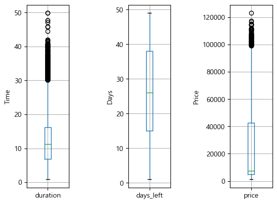
duration과 price에만 이상치가 있음을 확인할 수 있다.
04) 이상치 처리하기
결측치 처리 방식과 동일하다.
# 원본 복사
df_origin = df.copy()
(1) 이상치 데이터 삭제하기
# 신뢰도 95% 기준 이상치 Index 추출하기
outlier = df[(abs((df['price']-df['price'].mean())/df['price'].std())) > 1.96].index

# 추출한 인덱스의 행 삭제해서 clean_df 만들기
clean_df = df.drop(outlier)
clean_df.info()

# <class 'pandas.core.frame.DataFrame'>
# Index: 287660 entries, 0 to 300146
# Data columns (total 11 columns):
#  #   Column            Non-Null Count   Dtype
# ---  ------            --------------   -----
#  0   airline           287660 non-null  object
#  1   flight            287660 non-null  object
#  2   source_city       287660 non-null  object
#  3   departure_time    287660 non-null  object
#  4   stops             287660 non-null  object
#  5   arrival_time      287660 non-null  object
#  6   destination_city  287660 non-null  object
#  7   class             287660 non-null  object
#  8   duration          287660 non-null  float64
#  9   days_left         287660 non-null  int64
#  10  price             287660 non-null  int64
# dtypes: float64(1), int64(2), object(8)
# memory usage: 26.3+ MB
# 결과 확인
plt.figure(figsize=(4,5))
# 상자 그래프로 이상치 제거 여부 확인하기
clean_df[['price']].boxplot()
plt.show()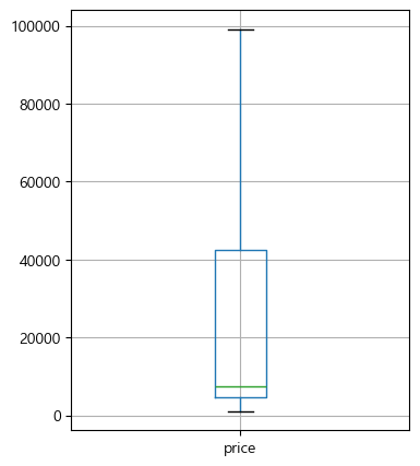
(2) 이상치 데이터 대체하기
def changeOutliers(x, column):
"""IQR 기준 이상치 대체하는 함수"""
# 제1사분위수
q1 = x[column].quantile(0.25)
# 제3사분위수
q3 = x[column].quantile(0.75)
# IQR의 1.5배수 IQR 구하기
iqr = 1.5 * (q3 - q1)
# 이상치 대체할 Min, Max 값 설정
Min = q1 - iqr
Max = q3 + iqr
# Max보다 큰 값은 Max로 작은 값은 Min으로 대체
x.loc[(x[column] > Max), column] = Max
x.loc[(x[column] < Min), column] = Min
return x
# price에 대하여 이상치 대체하기
clean_df = changeOutliers(df, 'price')
clean_df.info()
# <class 'pandas.core.frame.DataFrame'>
# RangeIndex: 300153 entries, 0 to 300152
# Data columns (total 11 columns):
# # Column Non-Null Count Dtype
# --- ------ -------------- -----
# 0 airline 300153 non-null object
# 1 flight 300153 non-null object
# 2 source_city 300153 non-null object
# 3 departure_time 300153 non-null object
# 4 stops 300153 non-null object
# 5 arrival_time 300153 non-null object
# 6 destination_city 300153 non-null object
# 7 class 300153 non-null object
# 8 duration 300153 non-null float64
# 9 days_left 300153 non-null int64
# 10 price 300153 non-null int64
# dtypes: float64(1), int64(2), object(8)
# memory usage: 25.2+ MBprint(f"price IQR Outliers > {findOutliers(clean_df, 'price')}") # price IQR Outliers > 0
# 결과 확인
plt.figure(figsize=(4,5))

# 상자 그래프로 이상치 제거 여부 확인하기
clean_df[['price']].boxplot()
plt.show()05) 구간화하기
구간화(binning)는 연속형 데이터를 특정 구간으로 나누어 범주형 또는 순위형으로 변환하는 방법을 말한다.
구간화하면 이상치로 발생 가능한 문제를 줄이고 결과에 대한 해석이 쉬워질 수 있다.
동일한 길이로 구간화하는 방법과 동일 개수로 구간화하는 방법이 있다.
(1) 동일 길이로 구간화하기
cut을 사용하면 구간을 사용자가 지정해서 쉽게 구간화할 수 있는데 구간화하고자 하는 값과 함께 bins, labels 파라미터를 반드시 같이 지정해 주어야 한다.
# 비행시간을 0-5, 5-10, 10 이상의 3개 구간으로 나누어 거리(distance) 칼럼 생성하기
df['distance'] = pd.cut(df['duration'], bins=[0,5, 10, df['duration'].max()], labels=['short', 'medium', 'long'])
df.head()

#   airline	 flight	 source_city departure_time	stops	arrival_time	destination_city	class	duration	days_left	price	distance
# 0	SpiceJet SG-8709 Delhi	     Evening	    zero	Night	        Mumbai	            Economy	2.17	    1	        5953	short
# 1	SpiceJet SG-8157 Delhi	     Early_Morning	zero	Morning	        Mumbai	            Economy	2.33	    1	        5953	short
# 2	AirAsia	 I5-764  Delhi	     Early_Morning	zero	Early_Morning	Mumbai	            Economy	2.17	    1	        5956	short
# 3	Vistara	 UK-995	 Delhi	     Morning	    zero	Afternoon	    Mumbai	            Economy	2.25	    1	        5955	short
# 4	Vistara	 UK-963	 Delhi	     Morning	    zero	Morning	        Mumbai	            Economy	2.33	    1	        5955	short
# 거리 칼럼의 빈도 분포
df['distance'].value_counts()
# distance
# long 169879
# medium 84761
# short 45513
# Name: count, dtype: int64(2) 동일한 개수로 구간화하기
qcut은 cut과 사용 방법이 동일하다. 다만, bins 대신 정수를 넣어 해당 구간만큼 동일한 양의 데이터가 들어가도록 구간화한다.
# 항공권 가격(price)을 4개 구간으로 동일하게 나누어 항공권 가격 비율 칼럼 생성
df['price_rate'] = pd.qcut(df['price'], 4, labels=['cheap', 'normal', 'expensive', 'too expensive'])
df.head()

# 	airline	 flight	 source_city departure_time	stops	arrival_time	destination_city	class	duration	days_left	price	distance	price_rate
# 0	SpiceJet SG-8709 Delhi	     Evening	    zero	Night	        Mumbai	            Economy	2.17	    1	        5953	short	    normal
# 1	SpiceJet SG-8157 Delhi	     Early_Morning	zero	Morning	        Mumbai	            Economy	2.33	    1	        5953	short	    normal
# 2	AirAsia	 I5-764	 Delhi	     Early_Morning	zero	Early_Morning	Mumbai	            Economy	2.17	    1	        5956	short	    normal
# 3	Vistara	 UK-995	 Delhi	     Morning	    zero	Afternoon	    Mumbai	            Economy	2.25	    1	        5955	short	    normal
# 4	Vistara	 UK-963	 Delhi	     Morning	    zero	Morning	        Mumbai	            Economy	2.33	    1	        5955	short	    normal
# 항공권 가격 비율 칼럼의 빈도분포 확인
df['price_rate'].value_counts()
# price_rate
# expensive 75584
# normal 75117
# cheap 75073
# too expensive 74379
# Name: count, dtype: int64Section 02 범주형 데이터 정제하기
01) 레이블 인코딩하기
(1) 판다스에서 레이블 인코딩하기
# 데이터 구간화 전 원본 불러오기
df = df_origin.copy()

# factorize로 airline 칼럼 레이블 인코딩하기
df['label_encoding'] = pd.factorize(df['airline'])[0].reshape(-1, 1)
df.head()
#   airline	 flight  source_city departure_time stops arrival_time	destination_city	class	duration	days_left	price	label_encoding
# 0	SpiceJet SG-8709 Delhi	     Evening	    zero  Night	        Mumbai	            Economy	2.17	    1	        5953	0
# 1	SpiceJet SG-8157 Delhi	     Early_Morning	zero  Morning	    Mumbai	            Economy	2.33	    1	        5953	0
# 2	AirAsia	 I5-764	 Delhi	     Early_Morning	zero  Early_Morning	Mumbai	            Economy	2.17	    1	        5956	1
# 3	Vistara	 UK-995	 Delhi	     Morning	    zero  Afternoon	    Mumbai	            Economy	2.25	    1	        5955	2
# 4	Vistara	 UK-963	 Delhi	     Morning	    zero  Morning	    Mumbai	            Economy	2.33	    1	        5955	2
# airline 칼럼과 새로 만들어진 label_encoding 칼럼의 빈도표 확인
print(df['airline'].value_counts())
# airline
# Vistara 127859
# Air_India 80892
# Indigo 43120
# GO_FIRST 23173
# AirAsia 16098
# SpiceJet 9011
# Name: count, dtype: int64
print(df['label_encoding'].value_counts())
# label_encoding
# 2 127859
# 5 80892
# 4 43120
# 3 23173
# 1 16098
# 0 9011
# Name: count, dtype: int64(2) 사이킷런으로 레이블 인코딩하기
from sklearn.preprocessing import LabelEncoder

# LabelEncoder로 airline 칼럼 레이블 인코딩하기
le = LabelEncoder()
df['airline_Label_Encoder'] = le.fit_transform(df['airline'])
df.head()
#   airline	 flight	 source_city  departure_time  stops  arrival_time  destination_city  class      duration  days_left	price	label_encoding	airline_Label_Encoder
# 0	SpiceJet SG-8709 Delhi	      Evening         zero	 Night	       Mumbai	         Economy	2.17	  1	        5953	0	            4
# 1	SpiceJet SG-8157 Delhi	      Early_Morning	  zero	 Morning	   Mumbai	         Economy	2.33	  1	        5953	0	            4
# 2	AirAsia	 I5-764	 Delhi	      Early_Morning	  zero	 Early_Morning Mumbai	         Economy	2.17	  1	        5956	1	            0
# 3	Vistara	 UK-995	 Delhi	      Morning	      zero	 Afternoon	   Mumbai	         Economy	2.25	  1	        5955	2	            5
# 4	Vistara	 UK-963	 Delhi	      Morning	      zero	 Morning	   Mumbai	         Economy	2.33	  1	        5955	2	            5
# airline 칼럼과 새로 만들어진 airline_Label_Encoder 칼럼의 빈도표 확인
print(df['airline'].value_counts())
# airline
# Vistara 127859
# Air_India 80892
# Indigo 43120
# GO_FIRST 23173
# AirAsia 16098
# SpiceJet 9011
# Name: count, dtype: int64
print(df['airline_Label_Encoder'].value_counts())
# airline_Label_Encoder
# 5 127859
# 1 80892
# 3 43120
# 2 23173
# 0 16098
# 4 9011
# Name: count, dtype: int64# 레이블 인코딩 디코딩하기
le.inverse_transform(df['airline_Label_Encoder']).reshape(-1, 1)
# array([['SpiceJet'],
# ['SpiceJet'],
# ['AirAsia'],
# ...,
# ['Vistara'],
# ['Vistara'],
# ['Vistara']], dtype=object)02) 원핫 인코딩하기
(1) 판다스에서 원핫 인코딩하기
# 레이블 인코딩 전 원본 데이터 불러오기
df = df_origin.copy()

# class 칼럼을 원핫 인코딩하기
pd.get_dummies(df['class'])

#   Business	Economy
# 0	False	    True
# 1	False	    True
# 2	False	    True
# 3	False	    True
# 4	False	    True

df = pd.get_dummies(df, columns=['class'])
df.head()
#   airline	    flight	source_city	departure_time	stops	arrival_time	destination_city	duration	days_left	price	class_Business	class_Economy
# 0	SpiceJet	SG-8709	Delhi	    Evening	        zero	Night	        Mumbai	            2.17	    1	        5953	False	        True
# 1	SpiceJet	SG-8157	Delhi	    Early_Morning	zero	Morning	        Mumbai	            2.33	    1	        5953	False	        True
# 2	AirAsia	    I5-764	Delhi	    Early_Morning	zero	Early_Morning	Mumbai	            2.17	    1	        5956	False	        True
# 3	Vistara	    UK-995	Delhi	    Morning	        zero	Afternoon	    Mumbai	            2.25	    1	        5955	False	        True
# 4	Vistara	    UK-963	Delhi	    Morning	        zero	Morning	        Mumbai	            2.33	    1	        5955	False	        True
(2) 사이킷런으로 원핫 인코딩하기
판다스의 get_dummies와 같이 바로 데이터프레임에 반영할 수 없어 원핫 인코딩 후 데이터를 추가하기 위해 추가하는 작업이 필요하다.
# 원본 데이터 불러오기
df = df_origin.copy()

from sklearn.preprocessing import OneHotEncoder

# OneHotEncoder로 원핫 인코딩하기
ohe = OneHotEncoder()
encoder = ohe.fit_transform(df['class'].values.reshape(-1, 1)).toarray()

# 원핫 인코딩 결과를 데이터프레임으로 만들기
df_ohe = pd.DataFrame(encoder, columns=["class_" + str(ohe.categories_[0][i]) for i in range(len(ohe.categories_[0]))])

# 원핫 인코딩 결과를 원본 데이터에 붙여넣기
pd.concat([df, df_ohe], axis=1).head()
#   airline     flight  source_city	departure_time	stops	arrival_time	destination_city	class	duration	days_left	price	class_Business	class_Economy
# 0	SpiceJet	SG-8709	Delhi	    Evening	        zero	Night	        Mumbai	            Economy	2.17	    1	        5953	0.0	            1.0
# 1	SpiceJet	SG-8157	Delhi	    Early_Morning	zero	Morning	        Mumbai	            Economy	2.33	    1	        5953	0.0	            1.0
# 2	AirAsia	    I5-764	Delhi	    Early_Morning	zero	Early_Morning	Mumbai	            Economy	2.17	    1	        5956	0.0	            1.0
# 3	Vistara	    UK-995	Delhi	    Morning	        zero	Afternoon	    Mumbai	            Economy	2.25	    1	        5955	0.0	            1.0
# 4	Vistara	    UK-963	Delhi	    Morning	        zero	Morning	        Mumbai	            Economy	2.33	    1	        5955	0.0	            1.0
Section 03 스케일링하기
01) 정규화하기
# 원핫인코딩 전 원본 데이터 불러오기
df = df_origin.copy()

# 수치형 데이터만 분리하여 데이터프레임 만들기
df_num = df[['duration', 'days_left', 'price']]

# 정규화 수식 적용하기
df_num = (df_num - df_num.min())/(df_num.max()-df_num.min())
df_num.head()

# 	duration	days_left	price
# 0	0.027347	0.0	        0.039749
# 1	0.030612	0.0	        0.039749
# 2	0.027347	0.0	        0.039773
# 3	0.028980	0.0	        0.039765
# 4	0.030612	0.0	        0.039765
# 요약 데이터로 정규화 적용 확인하기기
df_num.describe()
# duration days_left price
# count 300153.000000 300153.000000 300153.000000
# mean 0.232470 0.520932 0.162215
# std 0.146775 0.282521 0.186099
# min 0.000000 0.000000 0.000000
# 25% 0.122449 0.291667 0.030156
# 50% 0.212653 0.520833 0.051818
# 75% 0.313061 0.770833 0.339570
# max 1.000000 1.000000 1.00000002) 표준화하기
df_num = df[['duration', 'days_left', 'price']]

# 표준화 수식 적용하기
df_num = (df_num - df_num.mean())/df_num.std()
df_num.head()

#   duration	days_left	price
# 0	-1.397528	-1.843872	-0.658067
# 1	-1.375282	-1.843872	-0.658067
# 2	-1.397528	-1.843872	-0.657935
# 3	-1.386405	-1.843872	-0.657979
# 4	-1.375282	-1.843872	-0.657979
# 요약 데이터로 표준화 적용 확인하기
df_num.describe()
# duration days_left price
# count 3.001530e+05 3.001530e+05 3.001530e+05
# mean 7.726764e-17 9.393321e-17 -6.060207e-17
# std 1.000000e+00 1.000000e+00 1.000000e+00
# min -1.583847e+00 -1.843872e+00 -8.716567e-01
# 25% -7.495861e-01 -8.114997e-01 -7.096143e-01
# 50% -1.350141e-01 -3.503362e-04 -5.932152e-01
# 75% 5.490796e-01 8.845399e-01 9.530162e-01
# max 5.229282e+00 1.695689e+00 4.501823e+00# 기존의 duration, days_left, price 칼럼 삭제하기
df = df.drop(['duration', 'days_left', 'price'], axis=1)
# 표준화된 duration, days_left, price 칼럼 붙이기
df = pd.concat([df, df_num], axis=1)
df.head()
# airline flight source_city departure_time stops arrival_time destination_city class duration days_left price
# 0 SpiceJet SG-8709 Delhi Evening zero Night Mumbai Economy -1.397528 -1.843872 -0.658067
# 1 SpiceJet SG-8157 Delhi Early_Morning zero Morning Mumbai Economy -1.375282 -1.843872 -0.658067
# 2 AirAsia I5-764 Delhi Early_Morning zero Early_Morning Mumbai Economy -1.397528 -1.843872 -0.657935
# 3 Vistara UK-995 Delhi Morning zero Afternoon Mumbai Economy -1.386405 -1.843872 -0.657979
# 4 Vistara UK-963 Delhi Morning zero Morning Mumbai Economy -1.375282 -1.843872 -0.657979Section 04 변수 선택하기
01) 신규 변수 생성하기
(1) 하나의 데이터로 여러 개의 새로운 칼럼 만들기
# 항공기 기종을 제조사 코드와 모델명과 분리하는 split_flight 함수 만들기
def split_flight(flight):
    # "-"을 기준으로 앞쪽을 제조사 코드로 저장
    manufacture = flight.split('-')[0]
    # "-"을 기준으로 뒤쫏을 모델명으로 저장
    model = flight.split('-')[1]
    # 제조사 코드와 모델명을 반환
    return manufacture, model

# zip 함수를 사용해 튜플으로 묶어 새 칼럼으로 저장
df['manufacture'], df['model_num'] = zip(*df['flight'].apply(lambda x:split_flight(x)))
df.head()
# 	airline	    flight	source_city	departure_time	stops	arrival_time	destination_city	class	duration	days_left	price	    manufacture	model_num
# 0	SpiceJet	SG-8709	Delhi	    Evening	        zero	Night	        Mumbai	            Economy	-1.397528	-1.843872	-0.658067	SG	        8709
# 1	SpiceJet	SG-8157	Delhi	    Early_Morning	zero	Morning	        Mumbai	            Economy	-1.375282	-1.843872	-0.658067	SG	        8157
# 2	AirAsia	    I5-764	Delhi	    Early_Morning	zero	Early_Morning	Mumbai	            Economy	-1.397528	-1.843872	-0.657935	I5	        764
# 3	Vistara	    UK-995	Delhi	    Morning	        zero	Afternoon	    Mumbai	            Economy	-1.386405	-1.843872	-0.657979	UK	        995
# 4	Vistara	    UK-963	Delhi	    Morning	        zero	Morning	        Mumbai	            Economy	-1.375282	-1.843872	-0.657979	UK	        963
(2) 여러 개의 데이터로 하나의 새로운 칼럼 생성
# source_city, destination_city를 튜플로 묶어 route 칼럼 생성
df['route'] = df.apply(lambda x:(x['source_city'], x['destination_city']), axis=1)
df.head()

#   airline	    flight	source_city	departure_time	stops	arrival_time	destination_city	class	    duration	days_left	price	    manufacture	model_num	route
# 0	SpiceJet	SG-8709	Delhi	    Evening	        zero	Night	        Mumbai	            Economy	    -1.397528	-1.843872	-0.658067	SG	        8709	    (Delhi, Mumbai)
# 1	SpiceJet	SG-8157	Delhi	    Early_Morning	zero	Morning	        Mumbai	            Economy	    -1.375282	-1.843872	-0.658067	SG	        8157	    (Delhi, Mumbai)
# 2	AirAsia	    I5-764	Delhi	    Early_Morning	zero	Early_Morning	Mumbai	            Economy	    -1.397528	-1.843872	-0.657935	I5	        764	        (Delhi, Mumbai)
# 3	Vistara	    UK-995	Delhi	    Morning	        zero	Afternoon	    Mumbai	            Economy	    -1.386405	-1.843872	-0.657979	UK	        995	        (Delhi, Mumbai)
# 4 Vistara UK-963 Delhi Morning zero Morning Mumbai Economy -1.375282 -1.843872 -0.657979 UK 963 (Delhi, Mumbai)df.drop(['manufacture', 'model_num'], axis=1).head()02) 변수 선택하기