책 예제 사용합니다.
책: AICE Associate
책 예제 데이터1
책 예제 데이터2
Chapter 10 모델 성능 향상하기
Section 01 모델 하이퍼파라미터 튜닝 이해하기
01) 그리드 서치
(1) 그리드 서치 이해하기
(2) 그리드 서치 실습하기
GridSearchCV 하이퍼파라미터
- max_depth: 랜덤 포레스트 모델에서 각 의사결정나무의 최대 깊이
- max_features: 랜덤 포레스트 모델이 각 분할에서 시도할 수 있는 최대 특성 수
- n_estimators: 의사결정나무 수
- min_samples_leaf: 각 트리의 리프노드에 있어야 하는 최소 샘플 수
- min_samples_split: 각 트리의 내부 노드를 분할하는 데 필요한 최소 샘플 수
from sklearn.ensemble import RandomForestClassifier
from sklearn.model_selection import GridSearchCV

# Random Forest 분류기 생성하기
estimator = RandomForestClassifier()

# GridSearchCV 파라미터 저정하기
param_grid = {'max_depth':[3, 5, 10, None],
              'n_estimators':[10, 100, 200],
              'max_features':[1, 3, 5, 7],
              'min_samples_leaf':[1, 2, 3],
              'min_samples_split':[1, 2, 3]}

# GridSearchCV 생성 및 수행하기
gs_cv = GridSearchCV(estimator=estimator, param_grid=param_grid, scoring='accuracy', cv=3)

model = gs_cv.fit(X_train, y_train)
# 최적의 파라미터
print(f"Best Hyperparameter > {model.best_params_}")
print(f"Score > {model.best_score_}")시험 데이터셋으로 모델 성능을 평가한다.
# 모델 테스트 및 성능 확인하기
clf = model.best_estimator_
clf.fit(X_train, y_train)
print(f"테스트 정확도 > {clf.score(X_test, y_test)}")
02) 랜덤 서치
(1) 랜덤 서치 이해하기
(2) 랜덤 서치 실습하기
RandomizedSearchCV 하이퍼파라미터
- max_depth: 랜덤 포레스트 모델에서 각 의사결정나무의 최대 깊이
- n_estimators: 의사결정나무의 수
- criterion: 분할 품질을 측정하는 기능
- min_samples_leaf: 각 트리의 리프 노드에 있어야 하는 최소 샘플 수
- min_samples_split: 각 트리의 내부 노드를 분할하는데 필요한 최소 샘플 수
import numpy as np
from scipy.stats import randint
from sklearn.ensemble import RandomForestClassifierCV
from sklearn.model_selection import RandomizedSearchCV

# RandomForest 분류기 생성하기
estimator = RandomForestClassifierCV()

# RandomizedSearchCV 파라미터 범위 지정하기
param_distributions = {'max_depth':list(np.arage(3, 13, step=3)) + [None],
                       'n_estimators':np.arage(10, 320, step=100),
                       'max_features':randint(1, 7),
                       'criterion':['gini', 'entropy'],
                       'min_samples_leaf':randint(1, 4),
                       'min_samples_split':np.arange(2, 8, step=2)}

# RandomizedSearchCV 생성 및 수행하기
rs_cv = RandomizedSearchCV(estimator=estimator, param_distributions=param_distributions, n_iter=10, scoring='accuracy', n_jobs=-1, refit=True, cv=3)

model = rs_cv.fit(X_train, y_train)
# 최적의 파라미터
print(f"Best Hyperparameter > {model.best_params_}")
print(f"Score > {model.best_score_}")# 모델 테스트 및 성능 확인하기
clf = model.best_estimator_
clf.fit(X_train, y_train)
print(f"테스트 정확도 > {clf.score(X_test, y_test)}")Section 02 머신러닝 모델링 및 하이퍼파라미터 튜닝 실습하기
01) [회귀] 항공권 가격 예측 모델링하기
(1) 데이터 불러오기
import pandas as pd

cdf = pd.read_csv('./Clean_Dataset.csv')

# 학습 시간 단축을 위해 5,000건만 추출하기
cdf = cdf[:5000]

# 데이터 확인하기
cdf.head(1)

#   Unnamed: 0	airline	    flight	source_city	departure_time	stops	arrival_time	destination_city	class	duration	days_left	price
# 0	0	        SpiceJet	SG-8709	Delhi	    Evening	        zero	Night	        Mumbai	            Economy	2.17	    1	        5953
(2) 데이터 전처리하기
1) Unnamed 삭제 및 데이터 기초 통계 정보 확인하기
# Unnamed: 0 데이터 분포 확인하기
print(cdf['Unnamed: 0'].value_counts())
# Unnamed: 0
# 4999    1
# 0       1
# 1       1
# 2       1
# 3       1
#        ..
# 12      1
# 11      1
# 10      1
# 9       1
# 8       1
# Name: count, Length: 5000, dtype: int64

# Unnamed 칼럼 삭제하기
cdf = cdf.drop("Unnamed: 0", axis=1)
# 기초 통계 정보 확인하기
cdf.describe(include='all')
# airline flight source_city departure_time stops arrival_time destination_city class duration days_left price
# count 5000 5000 5000 5000 5000 5000 5000 5000 5000.000000 5000.000000 5000.000000
# unique 6 222 1 6 3 6 1 1 NaN NaN NaN
# top Vistara UK-819 Delhi Evening one Night Mumbai Economy NaN NaN NaN
# freq 1496 90 5000 1391 3619 1702 5000 5000 NaN NaN NaN
# mean NaN NaN NaN NaN NaN NaN NaN NaN 9.665682 14.216800 7589.786600
# std NaN NaN NaN NaN NaN NaN NaN NaN 7.247512 7.109536 4476.362204
# min NaN NaN NaN NaN NaN NaN NaN NaN 2.000000 1.000000 2409.000000
# 25% NaN NaN NaN NaN NaN NaN NaN NaN 2.330000 8.000000 4678.000000
# 50% NaN NaN NaN NaN NaN NaN NaN NaN 7.670000 14.000000 5955.000000
# 75% NaN NaN NaN NaN NaN NaN NaN NaN 14.080000 20.000000 10549.000000
# max NaN NaN NaN NaN NaN NaN NaN NaN 30.080000 26.000000 31260.0000002) Null 데이터 분석 및 처리하기
# info를 통해 Null 데이터 및 type이 있는지 1차 확인하기(isna 사용해도 됨)
cdf.info()
# <class 'pandas.core.frame.DataFrame'>
# RangeIndex: 5000 entries, 0 to 4999
# Data columns (total 11 columns):
#  #   Column            Non-Null Count  Dtype
# ---  ------            --------------  -----
#  0   airline           5000 non-null   object
#  1   flight            5000 non-null   object
#  2   source_city       5000 non-null   object
#  3   departure_time    5000 non-null   object
#  4   stops             5000 non-null   object
#  5   arrival_time      5000 non-null   object
#  6   destination_city  5000 non-null   object
#  7   class             5000 non-null   object
#  8   duration          5000 non-null   float64
#  9   days_left         5000 non-null   int64
#  10  price             5000 non-null   int64
# dtypes: float64(1), int64(2), object(8)
# memory usage: 429.8+ KB
3) airline 칼럼 분석 및 처리하기
# 첫 번째 칼럼이 의미 있는 칼럼인지 확인하기 위해 value_count로 분포 확인하기
cdf.airline.value_counts()
# 	        count
# airline
# Vistara	  1496
# Air_India	1311
# Indigo	  813
# GO_FIRST	801
# SpiceJet	296
# AirAsia	  283

# dtype: int64
항공사 수와 가격이 연관 있는지 그래프로 확인해본다.
import matplotlib.pyplot as plt
import seaborn as sns

# seaborn으로 막대 그래프 그리기

# 배경 사이즈 설정하기
plt.figure(figsize=(5, 5))

# 막대 사이즈 그리기
ax = sns.barplot(x='airline', y='price', data=cdf)

# 상단 타이틀 지정하기
ax.set(title='airline & price')

# 그래프 출력하기
plt.show()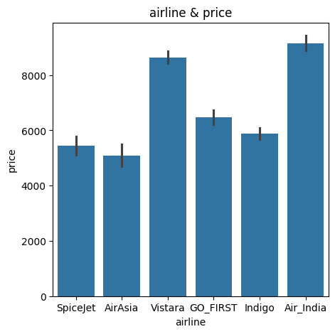
항공사별로 가격에 영향에 주는 것으로 추정되므로 airline 칼럼은 남겨둔다.
4) flight 칼럼 분석 처리하기
# 두 번째 flight 값 재확인하기
cdf.head(1)
#   airline	    flight	source_city	departure_time	stops	arrival_time	destination_city	class	duration	days_left	price
# 0	SpiceJet	SG-8709	Delhi	    Evening	        zero	Night	        Mumbai	            Economy	2.17	    1	        5953

# flight column 분포 확인하기
cdf.flight.value_counts()
# 	        count
# flight
# UK-819	90
# UK-879	62
# UK-899	61
# UK-705	61
# UK-835	60
# ...	...
# 6E-2901	2
# I5-881	2
# I5-744	1
# SG-8339	1
# SG-9974	1
# 222 rows × 1 columns


# dtype: int64
flight 칼럼은 충분히 유의미 하지만 '출발지', '도착지', '거리' 등이 있어 대체 가능한 것으로 보이므로 해당 칼럼은 삭제한다.
# flight 칼럼은 다른 칼럼과 의미가 중복되므로 삭제하기
cdf = cdf.drop('flight', axis=1)
5) 원핫 인코딩하기
# 원핫 인코딩을 위해 get_dummies 처리하기
dummies_cdf = pd.get_dummies(cdf, columns=["airline", "source_city", "departure_time", "stops", "arrival_time", "destination_city", "class"], drop_first=True)

# 인코딩 확인하기
print(f"{cdf.shape} -> {dummies_cdf.shape}")
# (5000, 10) -> (5000, 20)
6) 학습 데이터 만들기
# 데이터프레임에서 타깃 변수만 y로 추출하기
y = dummies_cdf.price
# 데이터프레임에서 타깃 변수를 제외한 입력 데이터셋 생성
x = dummies_cdf.drop('price', axis=1)
print(x.shape, y.shape)
# (5000, 20) (5000,)
x.head(1)
# duration days_left airline_Air_India airline_GO_FIRST airline_Indigo airline_SpiceJet airline_Vistara departure_time_Early_Morning departure_time_Evening departure_time_Late_Night departure_time_Morning departure_time_Night stops_two_or_more stops_zero arrival_time_Early_Morning arrival_time_Evening arrival_time_Late_Night arrival_time_Morning arrival_time_Night
# 0 2.17 1 False False False True False False True False False False False True False False False False True(3) 모델 학습하기
1) 머신러닝 라이브러리 불러오기
# 머신러닝 모델 생성하기
# 모델 생성 시 n_jobs 옵션이 있는 모델은 -1을 적용하여 동작시키는 것을 권유
lr = LinearRegression(n_jobs=-1)
dtr = DecisionTreeRegressor(random_state=42)
rtr = RandomForestRegressor(n_jobs=-1, random_state=42)
gbr = GradientBoostingRegressor(random_state=42)
xgbr = XGBRFRegressor(n_jobs=-1, random_state=42)
lgbm = LGBMRegressor(n_jobs=-1, random_state=42)
etr = ExtraTreesRegressor(n_jobs=-1, random_state=42)
lgbmr = LGBMRegressor(n_jobs=-1, random_state=42)
# 훈련 데이터 분할하기
x_train, x_test, y_train, y_test = train_test_split(x, y, test_size=0.3, random_state=42)
# shape 확인하기
x_train.shape, y_train.shape, x_test.shape, y_test.shape # ((3500, 19), (3500,), (1500, 19), (1500,))3) 머신러닝 모델 학습하기
%%time

# 머신러닝 모델 학습하기
lr.fit(x_train, y_train)
dtr.fit(x_train, y_train)
rfr.fit(x_train, y_train)
gbr.fit(x_train, y_train)
xgbr.fit(x_train, y_train)
etr.fit(x_train, y_train)
lgbmr.fit(x_train, y_train)
# Wall time: 3.17 s
4) 머신러닝 모델 성능 비교하기
from sklearn.metrics import r2_score, mean_squared_error
import numpy as np

# 리스트에 모델 입력하기
models = [lr, dtr, rfr, gbr, xgbr, etr, lgbmr]
r2_score_list, rmse_score_list = [], []

# 모델 결과 확인하기
for model in models:
  pred = model.predict(x_test)
  r2_score_list.append(round(r2_score(y_test, pred), 5))

  # squared를 False로 하면 RMSE가 됨
  mse2 = mean_squared_error(y_test, pred)
  rmse_score_list.append(round(np.sqrt(mse2), 5))

r2_score_df = pd.DataFrame([r2_score_list, rmse_score_list], columns=['lr', 'dtr', 'rfr', 'gbr', 'xgbr', 'etr', 'lgbmr'], index=["r2", "rmse"])
r2_score_df

#       lr	        dtr	        rfr	        gbr	        xgbr	    etr	        lgbmr
# r2	0.63056	    0.64306	    0.79672	    0.78557	    0.75211	    0.71466	    0.80882
# rmse	2691.02206	2645.11427	1996.13303	2050.16496	2204.32121	2364.98124	1935.80469
LGBM이 가장 좋은 성능을 보여준다.
(4) 최적의 파라미터 찾기
from sklearn.model_selection import GridSearchCV

# 비교 하이퍼파라미터 선정하기
param_grid = {'learning_rate': [0.1, 0.01, 0.003], 'colsample_bytree':[0.5, 0.7], 'max_depth':[20, 30, 40]}

# 최적 하이퍼파라미터 검색하기
cv_lgbmr = GridSearchCV(lgbmr, param_grid=param_grid, cv=5, verbose=1)
cv_lgbmr.fit(x_train, y_train)

# 최적 하이퍼파라미터 조합 확인하기
print(cv_lgbmr.best_params_) # {'colsample_bytree': 0.7, 'learning_rate': 0.1, 'max_depth': 20}

# 최적 파이퍼 파라미터 결과 확인하기 - 예측 정확도 확인하기
cv_lgbmr.best_score_ # np.float64(0.8036925831129313)
# 머신러닝 모델 검증하기
# 최적의 하이퍼파라미터로 재학습하기
best_lgbmr = LGBMRegressor(max_depth=20, learning_rate=0.1, colsample_bytree=0.7, n_jobs=-1, random_state=42)
best_lgbmr.fit(x_train, y_train)
# 모델 성능 검증하기
b_pred = best_lgbmr.predict(x_test)
print(f"r2 > {round(r2_score(y_test, b_pred), 5)}") # r2 > 0.80368
print(f"rmse > {round(np.sqrt(mean_squared_error(y_test, b_pred)), 5)}") # rmse > 1961.699780.80882 -> 0.80368 으로 앞선 결과보다 성능이 향상된 걸 볼 수 있다.
# RandomizedSearchCV로 최적 파라미터 구하는 방법
from sklearn.model_selection import RandomizedSearchCV

# 비교 파라미터 선정하기 RandomizedSearchCV로 최적 파라미터 구하는 방법
from sklearn.model_selection import RandomizedSearchCV

# 비교 파라미터 선정하기
param_dists = {'learning_rate':[0.1, 0.01, 0.003], 'colsample_bytree':[0.5, 0.7], 'max_depth':[20, 30, 40]}

# 최적 파라미터 검색하기
cv_lgbmr = RandomizedSearchCV(estimator=lgbmr, param_distributions=param_dists, n_iter=500, cv=5, verbose=1)

cv_lgbmr.fit(x_train, y_train)

# 최적 파라미터 조합 확인하기
print(cv_lgbmr.best_params_) # {'max_depth': 20, 'learning_rate': 0.1, 'colsample_bytree': 0.7}
02) [분류] 항공사 고객만족 여부 예측 모델링
(1) 데이터 불러오기
import pandas as pd

# 데이터 불러오기
cdf = pd.read_csv("./Invistico_Airline.csv")
cdf = cdf[:5000]

# 모든 칼럼을 표시하도록 설정
pd.set_option("display.max_columns", None)
(2) 데이터 전처리하기
타깃 변수인 satisfaction 칼럼에 있는 레이블 분포 확인한다.
print(cdf['satisfaction'].value_counts())
# satisfaction
# satisfied       2869
# dissatisfied    2131
# Name: count, dtype: int64

cdf['satisfaction'].value_counts().plot(kind='bar')
plt.show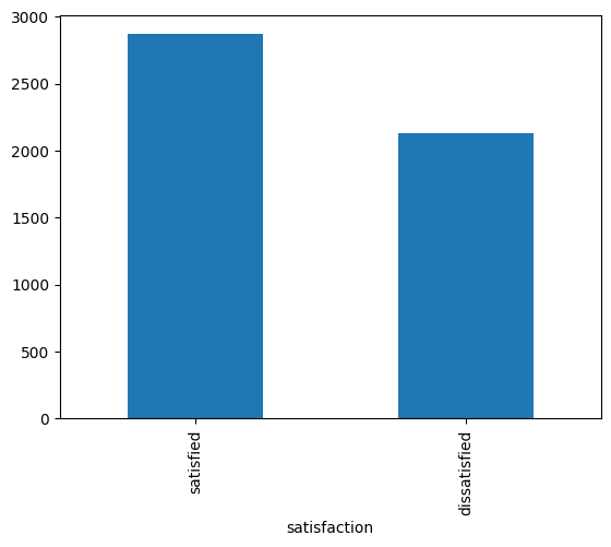
55:45 비율이므로 불균형 처리를 하지 않는다.
2) null 데이터 처리하기
cdf.info()
# <class 'pandas.core.frame.DataFrame'>
# RangeIndex: 5000 entries, 0 to 4999
# Data columns (total 23 columns):
#  #   Column                             Non-Null Count  Dtype
# ---  ------                             --------------  -----
#  0   satisfaction                       5000 non-null   object
#  1   Gender                             5000 non-null   object
#  2   Customer Type                      5000 non-null   object
#  3   Age                                5000 non-null   int64
#  4   Type of Travel                     5000 non-null   object
#  5   Class                              5000 non-null   object
#  6   Flight Distance                    5000 non-null   int64
#  7   Seat comfort                       5000 non-null   int64
#  8   Departure/Arrival time convenient  5000 non-null   int64
#  9   Food and drink                     5000 non-null   int64
#  10  Gate location                      5000 non-null   int64
#  11  Inflight wifi service              5000 non-null   int64
#  12  Inflight entertainment             5000 non-null   int64
#  13  Online support                     5000 non-null   int64
#  14  Ease of Online booking             5000 non-null   int64
#  15  On-board service                   5000 non-null   int64
#  16  Leg room service                   5000 non-null   int64
#  17  Baggage handling                   5000 non-null   int64
#  18  Checkin service                    5000 non-null   int64
#  19  Cleanliness                        5000 non-null   int64
#  20  Online boarding                    5000 non-null   int64
#  21  Departure Delay in Minutes         5000 non-null   int64
#  22  Arrival Delay in Minutes           4973 non-null   float64
# dtypes: float64(1), int64(17), object(5)
# memory usage: 898.6+ KB
# 결측치 행 삭제하기
cdf = cdf.dropna(axis=0)
cdf.info()
# <class 'pandas.core.frame.DataFrame'>
# Index: 4973 entries, 0 to 4999
# Data columns (total 23 columns):
# # Column Non-Null Count Dtype
# --- ------ -------------- -----
# 0 satisfaction 4973 non-null object
# 1 Gender 4973 non-null object
# 2 Customer Type 4973 non-null object
# 3 Age 4973 non-null int64
# 4 Type of Travel 4973 non-null object
# 5 Class 4973 non-null object
# 6 Flight Distance 4973 non-null int64
# 7 Seat comfort 4973 non-null int64
# 8 Departure/Arrival time convenient 4973 non-null int64
# 9 Food and drink 4973 non-null int64
# 10 Gate location 4973 non-null int64
# 11 Inflight wifi service 4973 non-null int64
# 12 Inflight entertainment 4973 non-null int64
# 13 Online support 4973 non-null int64
# 14 Ease of Online booking 4973 non-null int64
# 15 On-board service 4973 non-null int64
# 16 Leg room service 4973 non-null int64
# 17 Baggage handling 4973 non-null int64
# 18 Checkin service 4973 non-null int64
# 19 Cleanliness 4973 non-null int64
# 20 Online boarding 4973 non-null int64
# 21 Departure Delay in Minutes 4973 non-null int64
# 22 Arrival Delay in Minutes 4973 non-null float64
# dtypes: float64(1), int64(17), object(5)
# memory usage: 932.4+ KB27행이 삭제 됐다.
3) 학습 데이터 만들기
# 레이블 데이터 y를 나누기
# cdf 데이터프레임에서 label만 y로 추출
y = cdf.satisfaction

# satisfaction 칼럼 삭제하고 입력 데이터 만들기
x = cdf.drop("satisfaction", axis=1)

# 데이터 크기 확인하기
x.shape, y.shape # ((4973, 22), (4973,))
4) 원핫 인코딩하기
x.head(1)

#   Gender	Customer Type	Age	Type of Travel	Class	Flight Distance	Seat comfort	Departure/Arrival time convenient	Food and drink	Gate location	Inflight wifi service	Inflight entertainment	Online support	Ease of Online booking	On-board service	Leg room service	Baggage handling	Checkin service	Cleanliness	Online boarding	Departure Delay in Minutes	Arrival Delay in Minutes
# 0	Female	Loyal Customer	65	Personal Travel	Eco	    265	            0	            0	                                0	            2	            2	                    4	                    2	            3	                    3	                0	                3	                5	            3	        2	            0	                        0.0
# get_dummies 함수를 활용해 object 유형 칼럼 원핫 인코딩하기
x_gd = pd.get_dummies(x, columns=x.select_dtypes('object').columns, drop_first=False)
x_gd.info()
# <class 'pandas.core.frame.DataFrame'>
# Index: 4973 entries, 0 to 4999
# Data columns (total 25 columns):
# # Column Non-Null Count Dtype
# --- ------ -------------- -----
# 0 Age 4973 non-null int64
# 1 Flight Distance 4973 non-null int64
# 2 Seat comfort 4973 non-null int64
# 3 Departure/Arrival time convenient 4973 non-null int64
# 4 Food and drink 4973 non-null int64
# 5 Gate location 4973 non-null int64
# 6 Inflight wifi service 4973 non-null int64
# 7 Inflight entertainment 4973 non-null int64
# 8 Online support 4973 non-null int64
# 9 Ease of Online booking 4973 non-null int64
# 10 On-board service 4973 non-null int64
# 11 Leg room service 4973 non-null int64
# 12 Baggage handling 4973 non-null int64
# 13 Checkin service 4973 non-null int64
# 14 Cleanliness 4973 non-null int64
# 15 Online boarding 4973 non-null int64
# 16 Departure Delay in Minutes 4973 non-null int64
# 17 Arrival Delay in Minutes 4973 non-null float64
# 18 Gender_Female 4973 non-null bool
# 19 Gender_Male 4973 non-null bool
# 20 Customer Type_Loyal Customer 4973 non-null bool
# 21 Type of Travel_Personal Travel 4973 non-null bool
# 22 Class_Business 4973 non-null bool
# 23 Class_Eco 4973 non-null bool
# 24 Class_Eco Plus 4973 non-null bool
# dtypes: bool(7), float64(1), int64(17)
# memory usage: 772.2 KB5) 레이블 인코딩하기
from sklearn.model_selection import train_test_split
from sklearn.preprocessing import LabelEncoder

# train_test_split 수행하기
x_train, x_test, y_train, y_test = train_test_split(x_gd, y, stratify=y, test_size=0.3, random_state=42)

# 레이블 인코더 생성하기
le = LabelEncoder()

# fit으로 y_train 값마다 0, 1을 부여하는 규칙 생성
le.fit(y_train)

# y_train을 레이블 인코딩하기
le_y_train = le.transform(y_train)

# y_test를 레이블 인코딩하기
le_y_test = le.transform(y_test)

# 인코딩이 수행된 결과 확인하기
print(f"인코딩 후 데이터 > {le_y_train}") # 인코딩 후 데이터 > [1 1 1 ... 1 0 1]

# 레이블별로 어떤 값이 부여되어 있는지 규칙 확인
print(f"인코딩 클래스 확인 > {le.classes_}") # 인코딩 클래스 확인 > ['dissatisfied' 'satisfied']

# 인코딩된 데이터를 디코딩했을 때 데이터 확인
print(f"디코딩 후 데이터 > {le.inverse_transform(le_y_train)}") # 디코딩 후 데이터 > ['satisfied' 'satisfied' 'satisfied' ... 'satisfied' 'dissatisfied' 'satisfied']
(3) 모델 학습하기
from sklearn.linear_model import LogisticRegression
from sklearn.tree import DecisionTreeClassifier
from sklearn.ensemble import RandomForestClassifier, GradientBoostingClassifier, ExtraTreesClassifier
from xgboost import XGBRFClassifier
from lightgbm import LGBMClassifier

# 모델 생성하기
lr = LogisticRegression()
dtc = DecisionTreeClassifier(random_state=42)
rfc = RandomForestClassifier(random_state=42)
gbc = GradientBoostingClassifier(random_state=42)
xgbc = XGBRFClassifier(random_state=42)
etc = ExtraTreesClassifier(random_state=42)
lgbmc = LGBMClassifier(random_state=42)

# 모델 학습하기
lr.fit(x_train, le_y_train)
dtc.fit(x_train, le_y_train)
rfc.fit(x_train, le_y_train)
gbc.fit(x_train, le_y_train)
xgbc.fit(x_train, le_y_train)
etc.fit(x_train, le_y_train)
lgbmc.fit(x_train, le_y_train)

# 순서대로 적용할 모델을 리스트에 저장하기
models = [lr, dtc, rfc, gbc, xgbc, etc, lgbmc]

# for문을 활용해 학습 모델별 Score를 리스트에 저장하기
acc_train_list, acc_test_list = [], []

# 학습 모델별 Score를 리스트에 저장하기
for model in models:
  acc_train_list.append(round(model.score(x_train, le_y_train), 5))
  acc_test_list.append(round(model.score(x_test, le_y_test), 5))

# 모델별 정확도 출력하기
for i in range(len(models)):
  print(f"학습 모델 > {models[i]}")
  print(f"train 정확도 > {acc_train_list[i]}")
  print(f"test 정확도 > {acc_test_list[i]}")
  print("--------")

#   학습 모델 > LogisticRegression()
# train 정확도 > 0.81011
# test 정확도 > 0.81769
# --------
# 학습 모델 > DecisionTreeClassifier(random_state=42)
# train 정확도 > 1.0
# test 정확도 > 0.99933
# --------
# 학습 모델 > RandomForestClassifier(random_state=42)
# train 정확도 > 1.0
# test 정확도 > 0.99933
# --------
# 학습 모델 > GradientBoostingClassifier(random_state=42)
# train 정확도 > 1.0
# test 정확도 > 0.99933
# --------
# 학습 모델 > XGBRFClassifier(base_score=None, booster=None, callbacks=None,
#                 colsample_bylevel=None, colsample_bytree=None, device=None,
#                 early_stopping_rounds=None, enable_categorical=False,
#                 eval_metric=None, feature_types=None, gamma=None,
#                 grow_policy=None, importance_type=None,
#                 interaction_constraints=None, max_bin=None,
#                 max_cat_threshold=None, max_cat_to_onehot=None,
#                 max_delta_step=None, max_depth=None, max_leaves=None,
#                 min_child_weight=None, missing=nan, monotone_constraints=None,
#                 multi_strategy=None, n_estimators=None, n_jobs=None,
#                 num_parallel_tree=None, objective='binary:logistic',
#                 random_state=42, reg_alpha=None, ...)
# train 정확도 > 0.99914
# test 정확도 > 0.99799
# --------
# 학습 모델 > ExtraTreesClassifier(random_state=42)
# train 정확도 > 1.0
# test 정확도 > 0.99933
# --------
# 학습 모델 > LGBMClassifier(random_state=42)
# train 정확도 > 1.0
# test 정확도 > 1.0
# --------
(4) 최적의 하이퍼파라미터 찾기
1) 그리드 서치하기
# param_grid를 정의해 각 파라미터별로 교차해 모든 학습 수행
param_grid = {'n_estimators':[50, 100, 200, 500], 'max_features':['sqrt', 'log2', None], 'max_depth':[10, 20, 30, 40, 50, None]}

# GridSearchCV
cv_rfc = GridSearchCV(estimator=rfc, param_grid=param_grid, n_jobs=-1, cv=5)
cv_rfc.fit(x_train, le_y_train)

# best_score
print(f"best_score > {round(cv_rfc.best_score_, 5)}") # best_score > 0.99943

# best_params
print(f"best_params > {cv_rfc.best_params_}") # best_params > {'max_depth': 10, 'max_features': 'sqrt', 'n_estimators': 50}
# 최적 하이퍼파라미터로 도출된 값을 모델에 입력
best_rfc = RandomForestClassifier(n_estimators=50, max_features=None, n_jobs=-1, max_depth=10)
# rfc 학습 수행
rfc.fit(x_train, le_y_train)
# 이전 하이퍼파라미터 설정 없이 수행했을 때 정확도
print("기존 모델 Test 정확도: 0.99933")
# 최적 하이퍼파라미터 입력 후 학습시킨 모델의 정확도 확인
print(f"최적화한 모델 Test 정확도 > {round(rfc.score(x_test, le_y_test), 5)}")
# 향상된 정확도 차이
print(f"{round(rfc.score(x_test, le_y_test)-1.0, 5)}")(5) 오차 행렬로 모델 평가하기
from sklearn.metrics import confusion_matrix, ConfusionMatrixDisplay, classification_report

# rfc 모델로, x_test를 예측한 값을 y_pred로 저장
y_pred = rfc.predict(x_test)

# 실제값 le_y_test(레이블 인코딩 해야 0, 1로 표현됨)와 예측값 y_pred 비교
cm = confusion_matrix(le_y_test, y_pred, labels=[0,1])
disp = ConfusionMatrixDisplay(confusion_matrix=cm, display_labels=[0, 1])
disp.plot()

# confusion matrix 출력
plt.show()

# confusion matrix를 통한 각종 지표 리포트로 출력
print(classification_report(le_y_test, y_pred))
#               precision    recall  f1-score   support

#            0       1.00      1.00      1.00       635
#            1       1.00      1.00      1.00       857

#     accuracy                           1.00      1492
#    macro avg       1.00      1.00      1.00      1492
# weighted avg       1.00      1.00      1.00      1492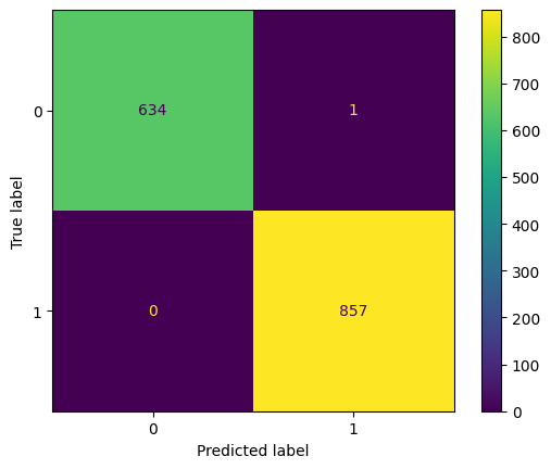
실제 dissatisfied인 데이터의 경우 제대로 예측한 것이 635개, 실제 satisfied인 경우 제대로 예측한 것은 857개로 제대로 예측한 것을 확인할 수 있다.