[Paper review] Why Attention Was All We Needed

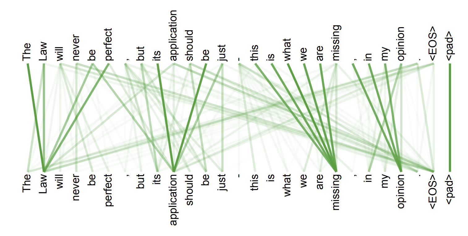
figure 1

A. Vaswani et al., “Attention Is All You Need”, NeurIPS, 2017

Earlier sequence models had limitations in handling sequential data. To address these issues, Vaswani et al. proposed the Transformer, a fully attention-based architecture that removes recurrence and convolution entirely. By using self-attention, the Transformer enables efficient parallel computation and stronger modeling of long-range dependencies.

Limitations of pre-transformer sequence models

• Parallelism limitation: Since recurrent models process tokens sequentially, they are difficult to train efficiently on GPUs.
• Gradient vanishing: Long sequences weaken gradients, limiting the ability to capture distant dependencies.
• The attention mechanism was used in previous models; however, it was only used alongside RNNs or CNNs.

The foundation: attention mechanism

In short, the attention function takes a query and a set of key–value pairs and measures how relevant each key is to the query, then returns a weighted sum of the values, giving higher weights to more relevant ones.

What are Q, K, and V?

• Query represents what the current token is looking for.
• Key represents what each token offers, describing the kind of information that token contains.
• Value carries the actual information that gets transferred to the output in proportion to how relevant its corresponding key is to the query.

  If you think of it like a search engine, Query is your search term, Keys are document titles, and Values are the actual contents of those documents.

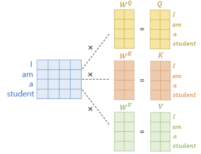
figure 2

The input $X \in \mathbb{R}^{n \times d_{\text{model}}}$ is linearly projected using learned weight matrices, producing $Q, K, V$ with dimensions $d_k$, $d_k$, and $d_v$, respectively.

Process of scaled dot-product attention

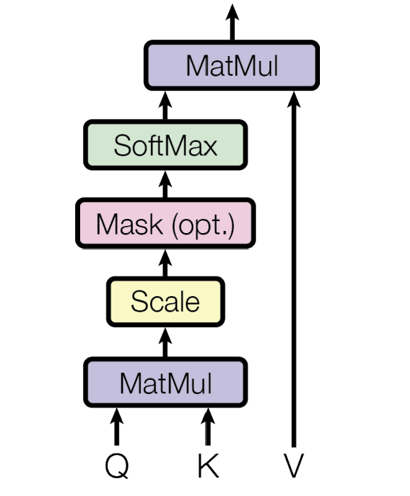
figure 3

1. MatMul: Compute the attention score matrix by $QK^\top$.
2. Scale: Divide by the scale factor $\sqrt{d_k}$.
   Scaling prevents large dot-product values from saturating the softmax, ensuring stable gradients and better training performance.
3. Mask (optional): Applied to prevent certain positions from being attended to (explained in more detail in the decoder section).
4. Softmax:
   $\text{softmax}(x_i) = \frac{e^{x_i}}{\sum_j e^{x_j}}$
   Converts the scaled scores into a probability distribution over all keys for each query.
   It produces attention weights that indicate how relevant each key is to the query — higher scores mean greater relevance.
5. MatMul (with V):
   Each query’s output becomes a weighted sum of all value vectors, where tokens that are more relevant to the query contribute more to the final representation.
   This allows the model to gather the most meaningful context for each query.

Finally, the formula represents all five steps above — from computing relevance to producing context-aware outputs.

Multi-head attention

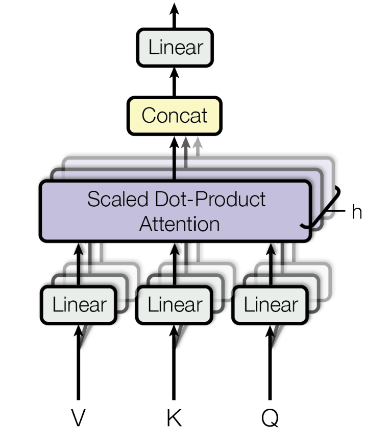
figure 4

Instead of a single attention, the Transformer uses multi-head attention to learn from different representation subspaces.
Each head has its own learnable projection matrices that produce $Q, K,$ and $V$ for each head:

Each head then applies scaled dot-product attention in parallel:

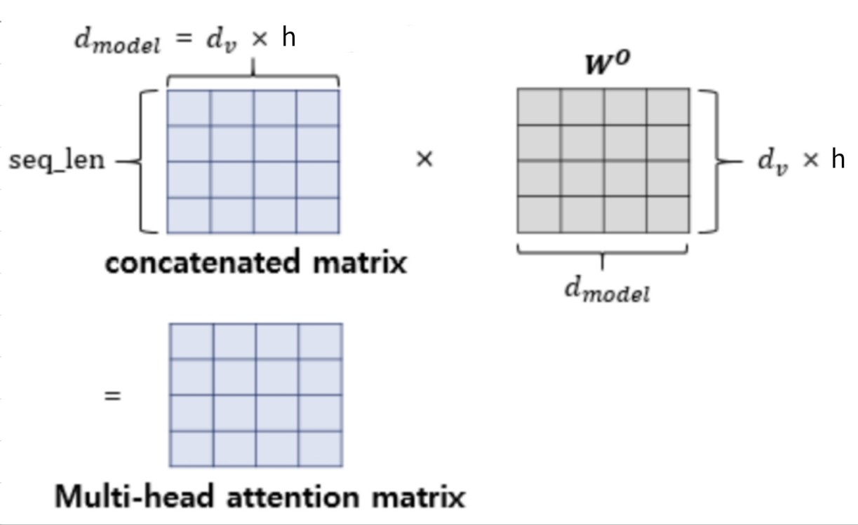
figure 5

Finally, the head outputs are concatenated and linearly projected back to $d_{\text{model}}$, ensuring consistency across all layers in the Transformer.

where

Why it helps:

• Diverse information: Multi-head attention allows the model to capture different types of relevance simultaneously. Each head specializes in focusing on distinct aspects of the sequence (e.g., syntax, semantics, or coreference), and their combination provides a richer overall understanding of context.
• Efficiency preserved: Although multiple heads are used, the total computational cost remains nearly the same as single-head attention since each head operates in a reduced dimension ($d_k = d_v = d_{\text{model}} / h$).

Transformer architecture

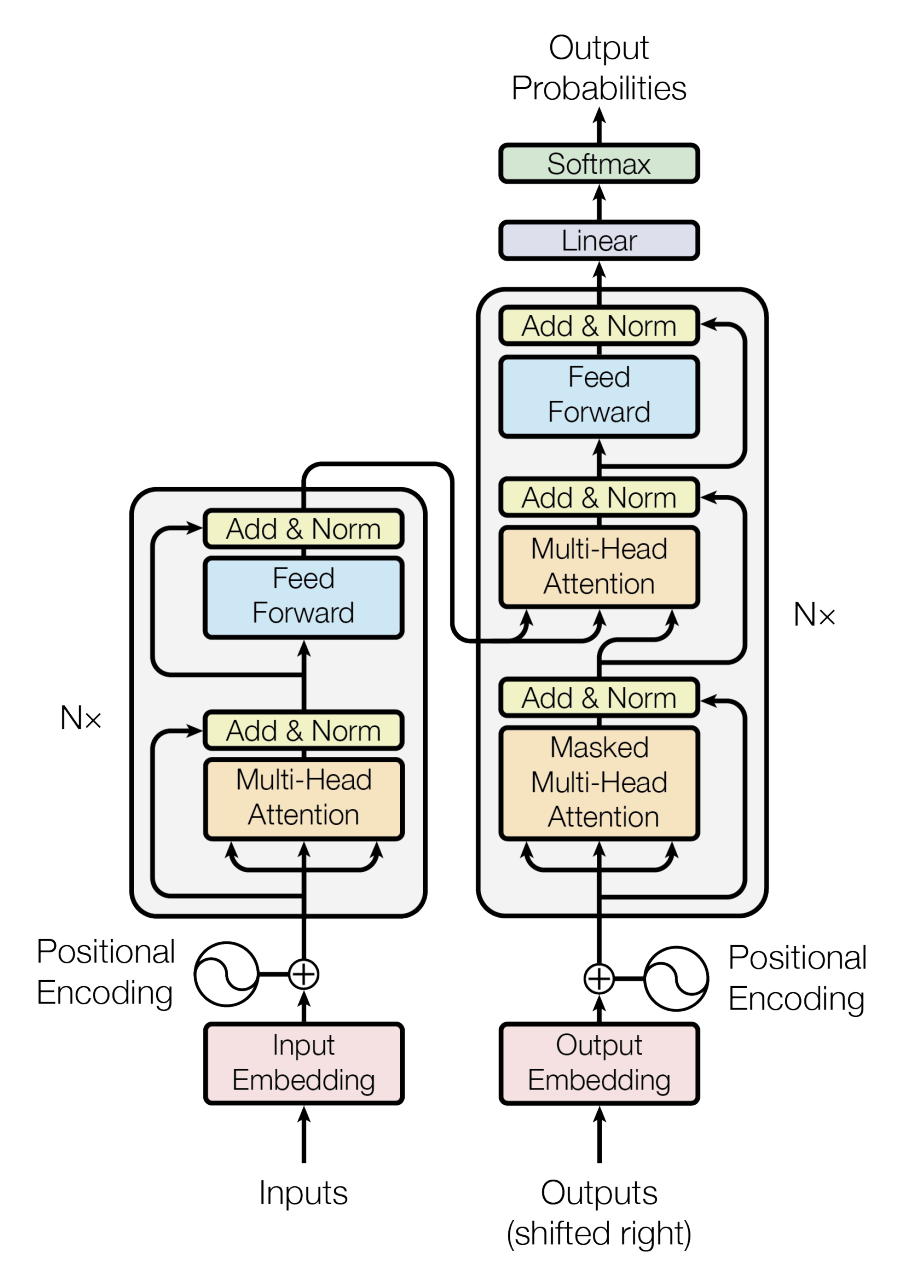
figure 6

Now that we understand attention and multi-head attention, we can look at the overall Transformer architecture, which is divided into two main parts: an encoder (on the left in the image) and a decoder (on the right).
Both are composed of a stack of $N = 6$ identical layers containing several sub-layers and components, and they share several of these sub-layers and components.

Common sub-layers & components

Positional encoding

Since the model has no recurrence or convolution, it needs a way to represent the order of tokens. To achieve this, sinusoidal positional encodings are added to the input embeddings at the bottoms of the encoder and decoder stacks:

where $pos$ is the position and $i$ is the dimension.
These encodings share the same dimensionality as embeddings ($d_{\text{model}}$), allowing them to be added directly.

Positional encoding enables the model to capture sequence order. The sinusoidal form was chosen because it allows the model to learn relative positions easily, since $PE_{pos+k}$ can be represented as a linear function of $PE_{pos}$.

Residual connections & layer normalization (Add & Norm)

Each sub-layer in both the encoder and decoder is wrapped with a residual connection followed by layer normalization:

where $x$ is the input to the sub-layer and $\text{Sublayer}(x)$ is the function implemented by the sub-layer itself.

Why it helps:

• Residual connection: Adds the sub-layer output to its input. It helps preserve information from earlier layers and stabilizes gradient flow.
• Layer normalization: Normalizes the summed result, stabilizing training and speeding up convergence.

To ensure that residual connections work seamlessly, every sub-layer and embedding layer in the model produces outputs with the same dimensionality ($d_{\text{model}}$).

Feed-forward network

Each layer in both the encoder and decoder includes a feed-forward network (FFN) that is applied independently at each position.

The FFN consists of two linear layers with a ReLU activation in between:

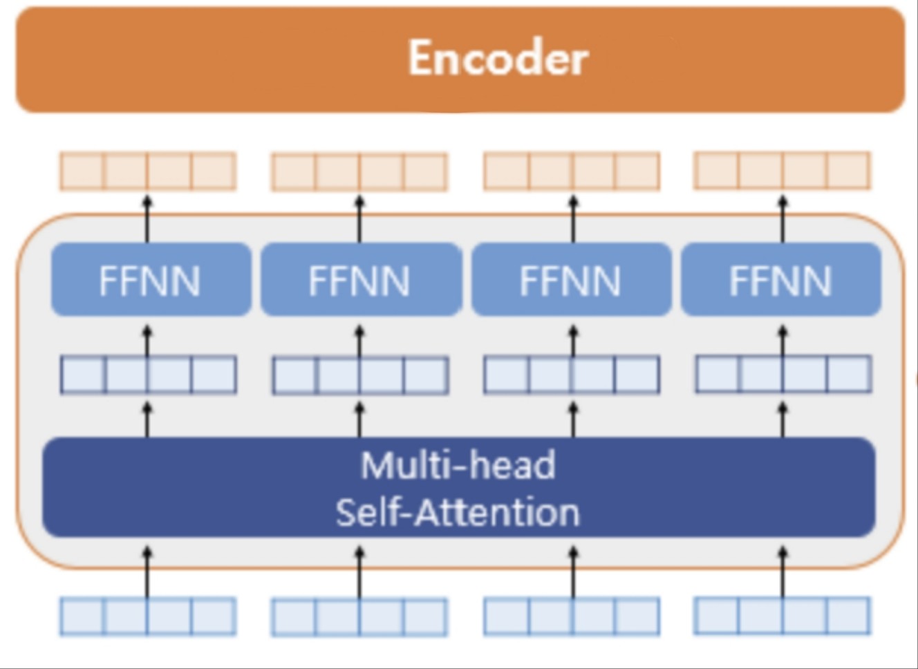
figure 7

The same weights are shared across all positions within a layer. However, the two layers inside the FFN have their own sets of weights, meaning parameters are not shared between them.

It first expands the representation to a higher dimension ($d_{\text{ff}}$) and then projects it back to the model dimension ($d_{\text{model}}$).

Encoder

figure 8

The encoder has six identical layers, and each layer contains two main sub-layers: multi-head self-attention and a feed-forward network (FFN).

• At the beginning (bottom of the figure8), the input embeddings are added to positional encodings.

  

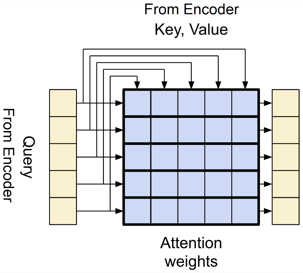
  figure 9

• The first sub-layer is multi-head self-attention. It's called self-attention because all queries, keys, and values come from the same source—the output of the previous layer in the encoder. Each position in the encoder can attend to all positions in the previous layer.
• The second sub-layer is the feed-forward network. After attention, each token's representation passes through the FFN, applied independently to every position.
• Add & Norm: Each sub-layer is wrapped with residual connections and normalization.

Decoder

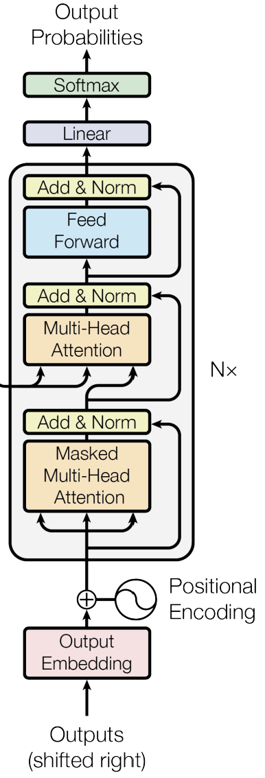
figure 10

The decoder also has six identical layers, but each layer contains three main sub-layers. It generates the output sequence one token at a time, using previously predicted tokens as context.

• At the beginning (bottom of the figure10), the output embeddings are added to positional encodings.

  

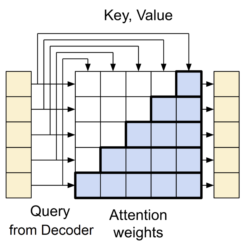
  figure 11

• The first sub-layer is masked multi-head self-attention. It is similar to the encoder’s self-attention, but the key difference is the mask that prevents each position from attending to future tokens. This preserves the auto-regressive property, ensuring the model only sees tokens up to the current position.

  

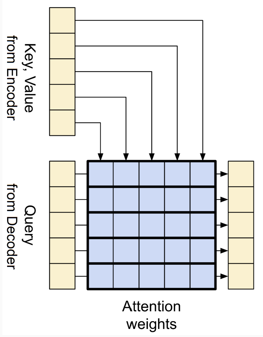
  figure 12

• The second sub-layer is encoder-decoder attention. Here, the queries come from the decoder’s previous sub-layer, while keys and values come from the encoder’s output. This allows every position in the decoder to attend to all positions in the input sequence, integrating the encoded information into the generation process.

• The third sub-layer is the feed-forward network. Same as in the encoder, each token's representation passes through the FFN.

• Add & Norm: Same as in the encoder, each sub-layer is wrapped with residual connections and normalization.

Why self-attention is better

The table below compares self-attention, recurrent, and convolutional layers in terms of their efficiency and ability to model long-range relationships. Here’s why self-attention stands out:

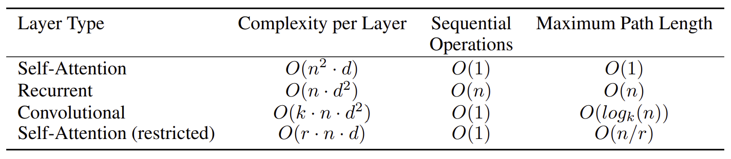
figure 13

1. Computational efficiency: Self-attention has lower per-layer cost than recurrent and convolutional layers in most practical cases.
2. Better parallelization: Self-attention connects all positions at once with fewer sequential operations, allowing full parallelization and much faster training.
3. Long-range dependencies: Self-attention directly connects any two positions in the sequence, making it easier to learn relationships between distant tokens. Recurrent and convolutional layers require multiple steps to connect distant positions, making them less effective at capturing global context.

Training & results

Training setup

The Transformer was trained on the WMT 2014 English–German (4.5M sentence pairs) and English–French (36M sentence pairs) datasets.
Sentences were tokenized using Byte Pair Encoding (BPE) to reduce vocabulary size and handle rare words efficiently.

Training used the Adam optimizer, along with regularization methods such as dropout (rate = 0.1) and label smoothing (ε = 0.1) to improve generalization and prevent overfitting.

Results

The Transformer achieved state-of-the-art performance on major translation benchmarks:

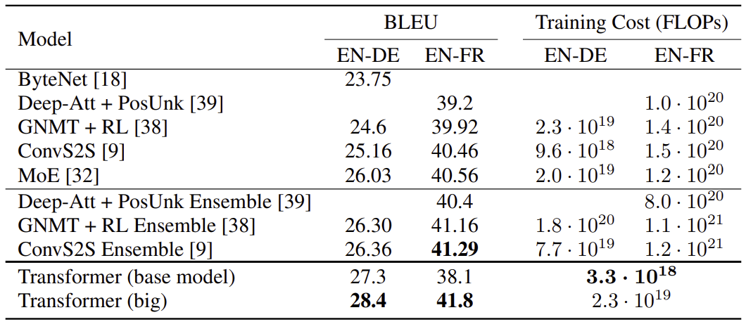
figure 14

Even the base model outperformed previous RNN and CNN models at far lower training cost.

Generalization

Beyond translation, the Transformer also performed well on English constituency parsing, showing that its attention-based architecture generalizes effectively to other sequence modeling tasks.

In short, the Transformer trained faster, cost less, and achieved higher accuracy than all prior sequence models—marking a major shift in deep learning architecture design.

Discussions

While the Transformer achieved remarkable results, it also introduced several challenges that motivated later research:

• Quadratic complexity in attention:
  The self-attention mechanism compares every token with every other token, causing quadratic growth in memory and computation as the sequence length increases. This makes Transformers inefficient for very long sequences like documents or videos.
  → I think the computational cost could be reduced from quadratic to near-linear by designing more efficient attention mechanisms.

• Fixed sequence length:
  The model relies on positional encodings with a fixed size, meaning it cannot naturally process sequences longer than those it was trained on. This limits its ability to handle dynamic or streaming data efficiently.
  → I think using relative positional encodings instead of fixed positional encodings allows the model to generalize better to sequences longer than those seen during training.

References

• Figure 1, 3, 4, 6, 8, 10, 13, 14 are taken or adapted from A. Vaswani et al., “Attention Is All You Need”, NeurIPS, 2017
• Figure 2, 5, 7 are adapted from Bryce, Eddie. 딥 러닝을 이용한 자연어 처리 입문.
• Figure 9, 11, 12 are adapted from PyLessons. “Attention layers in Transformer.” PyLessons tutorial blog, August 07, 2023.