- WGAN
- WGAN propose using the Wassertein distance to measure the distance between the two distribution.
1. Why Wasserstein is better than Js or KL?
(1) suppose that we have two probaility distribution P and Q
다음과 같이 distribution이 겹치지 않는 두 개의 joint propability distribution이 있다고 가정해보자.
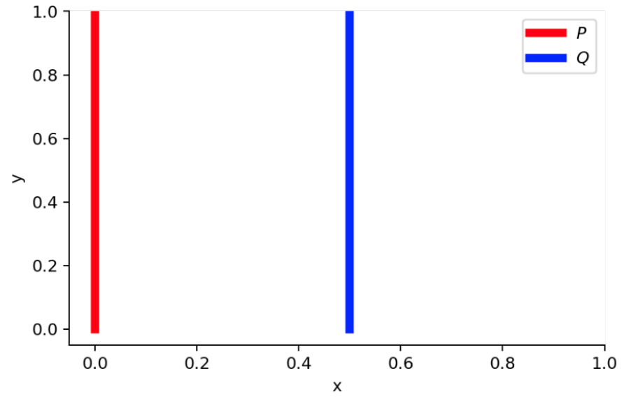
- ∀(x,y)∈P,x=0 and y∼U(0,1)
- ∀(x,y)∈Q,x=θ,0≤θ≤1, and y∼U(0,1)
(2) when θ=0
다음과 같은 조건에서 KL divergence 와 JS divergence를 구해보면,
- DKL(P∥Q)=∑x=0,y∼U(0,1)1⋅log01=+∞
- DKL(Q∥P)=∑x=θ,y∼U(0,1)1⋅log01=+∞
- DJS(P,Q)=21(∑x=0,y∼U(0,1)1⋅log211+∑x=0,y∼U(0,1)1⋅log211)=log2
으로 Gradient가 0인 것을 확인할 수 있다.
하지만, Wasserstein distance의 경우에는 2개의 distribution을 가장 가까이 겹치게 하는 방법은 line을 따라서 옮기는 것이므로,
- W(P,Q)=∣θ∣
(3) when θ=0
- DKL(P∥Q)=DKL(Q∥P)=DJS(P,Q)=0
- W(P,Q)=0=∣θ∣
(2), (3)의 경우를 통해서 보았을 때, wasserstien distance가 KL divergence와 JS divergence보다 훨씬 smooth한 distance measure를 가지고 있는 것을 알 수 있다.
2. Kantorovich-Rubinstein duality
우리는 지금까지 2개의 distribution이 겹치지 않는 경우에 Wasserstien distance가 KL, JS divergence 보다 distribution measure 측면에서 훨씬 유의미한 정보를 제공하는 것을 확인하였다.
하지만, W(pr,pθ)=infγ∼Π(pr,pθ)E(x,y)∼γ[∥x−y∥] 에서
γ∼Π(pr,pθ)는 가능한 모든 joint distribution의 set이기 때문에,
이를 모두 고려하여 wassertein distance를 구한다는 것은 사실상 불가능하다.
이러한 primal problem을 풀기 위해 dual problem으로 바꿔서 문제를 해결하는 Kantorovish-Rubinstein duality가 등장한다.
(1) Highly intractable term in inf
W(Pr,Pg)=infγ∈Π(Pr,Pg)E(x,y)∼γ[∥x−y∥] 는 highly intractable하다.
따라서 Kantorovish-Rubinstein duality를 통해, Lipschitz continuous 조건을 만족하는 '어떠한' function f:X→R를 통해서 다음과 같은 dual problem으로 문제를 해결한다.
- W(pr,pθ)=K1sup∥f∥L≤KEx∼pr[f(x)]−Ex∼pθ[f(x)]
이렇게 Wasserstein distance를 duaility를 통해서 다르게 정의할 수 있다. 그렇다면 f는 무엇인가?
(2) Find optimal f(x)
f는 말 그대로, Ex∼pr[f(x)]−Ex∼pθ[f(x)]의 값을 최대로 만족하는 '어떠한' function f이다.
이러한 f를 잘 '추정' 하기 위해서 parameter w를 가지는 neural network를 사용하여 다음과 같은 수식을 만족시키는 fw를 추정해준다. (neural network 는 universal function approximator 이기 때문에 neural net을 사용하여 f를 추정한다.)
maxw∈WEx∼pr[fw(x)]−Ex∼pθ[fw(x)]≤sup∥f∥L≤KEx∼pr[f(x)]−Ex∼pθ[f(x)]=K⋅W(Pr,Pθ)
우리는 그저 sup 형태로 존재하는 f(x)를 잘 추정하면 되기 때문에, 굳이 K에 대해 자세하게 알 필요가 없다.
-
maxw∈WEx∼pr[fw(x)]−Ex∼pθ[fw(x)] 을 만족하는 fw(x)를 찾기 위해 gradient를 구해준다.
-
∇w[fw(x)−f(gθ(z))] 를 통해서 sup problem의 solution인 f(x)를 추정해주는 fw(x)의 parameter w를 update한다.
(3) Generator update process
Neural network를 통해서 fw를 구한 다음, Generator의 parameter θ를 update 시켜준다.
∇θW(pr,pg)=∇θ(Ex∼pr[fw(x)]−Ez∼Z[fw(gθ(z))])=−Ez∼Z[∇θfw(gθ(z))]
(4) Weight Clipping
초기에 sup problem을 생각해보면, Kantorovish-Rubinstein duality를 통해서 Primal problem을 dual problem으로 끌고 간다. 이 때, Lipschitz Continuous를 만족해야 한다는 조건이 붙는다. Neural Network를 통해서 fw(x)를 추정할 때, fw(x)또한 Lipschitz Continuous를 만족해야 한다. Neural network에서 fw의 Gradient는 곧 weight이기 때문에, Weight Clipping 해주면 그 것 자체로 Lipschitz Continuous를 만족시키는 것이다. 따라서, Weight Clipping을 통해서 Lipschitz Countinuous를 만족시켜준다.
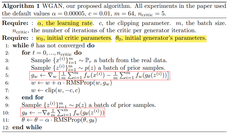
(5) Total training process
전체적인 Process의 pseudo code이다.
1. 우선, Earth Mover's distance optimization problem을 dual problem으로 바꾸어준다. 그 다음, 고정된 θ에서 Dual problem solution의 approximated function fw(x)를 training을 통해서서 찾아준다.
2. Wasserstein distance를 backprop해서 generator의 파라미터를 update 시켜준다.