Data Preparation & Exploration

박신영·2023년 3월 25일

DB 2_Porto Seguro's Safe Driver Prediction

목록 보기

1/1

🔶Introduction

✔️ PorteSeguro Competition data에 대한 good insight를 얻는 것이 목표
✔️ 운전자가 내년에 자동차 보험 청구를 시작할 확률을 예측하는 모델 구축
✔️ predict_proba 함수를 통해 확률 값 예측
✔️ Normalized Gini Coefficient를 평가지표로 사용

✔️ 메인 섹션
1. 데이터에 대한 시각적 영감
2. 메타데이터 정의
3. Descriptive 통계량
4. 불균형 classes 처리
5. 데이터의 quality 확인
6. Exploratory data visualization
7. Feature engineering
8. Feature 선택
9. Feature scaling

Information about data

train set 59만 개, test set 89만 개
feature가 비식별화 되어있어 난이도 높음(실제 기업 데이터는 보통 비식별화)
feature이 그루핑 되어 있음
- ind : 정수값 매핑
- reg : region
- car : 차에 관한 변수
- calc : 실수 값
target은 이전에 보험 청구가 있었으면 1, 아니면 0

Loading packages

import pandas as pd
import numpy as np
import matplotlib.pyplot as plt
import seaborn as sns
# matplotlib의 기본 scheme이 아닌 seaborn scheme을 세팅하기
# graph의 font size를 지정하지 않고 seaborn의 font_scale 사용하면 편리

from sklearn.impute import SimpleImputer
# 결측치 대체를 위한 라이브러리(Imputer->SimpleImputer로 업데이트)
from sklearn.preprocessing import PolynomialFeatures
from sklearn.preprocessing import StandardScaler
from sklearn.feature_selection import VarianceThreshold
from sklearn.feature_selection import SelectFromModel
from sklearn.utils import shuffle
from sklearn.ensemble import RandomForestClassifier

pd.set_option('display.max_columns', 100)

🔶데이터에 대한 시각적 영감

✔️ pandas는 테이블화 된 데이터 다루기 최적화, 많이 쓰이는 라이브러리
✔️ 데이터 셋의 간단한 통계적 분석 ~ 복잡한 처리들 사용 가능
✔️ 캐글에서 데이터셋은 보통 train과 test set으로 나뉘어짐

from google.colab import drive
drive.mount('/content/drive')

pwd

대회 데이터 설명의 발췌록
- 유사한 그룹의 feature는 ind, reg, car, calc 등의 피쳐이름과 같은 태그 지정됨
- bin ➡️ binary feature & cat ➡️ categorical feature
  - 지정 X feature 은 연속형 or 순서형
- 값이 -1이면 형상이 관측치에서 누락되었음을 의미(Null Value)
target 열은 해당 정책 소유자에 관한 클레임이 제기되었는지 여부를 나타냄

df_train = pd.read_csv('./drive/MyDrive/ECC 데과B/train_w2.csv')
df_test = pd.read_csv('./drive/MyDrive/ECC 데과B/test_w2.csv')
df_train.head()
# head()는 파일의 앞부분만 보여주는 것
# 괄호 안에 아무 입력이 없을 경우 기본인 5줄로 출력

index id target ps_ind_01 ps_ind_02_cat ps_ind_03 ps_ind_04_cat ps_ind_05_cat ps_ind_06_bin ps_ind_07_bin ps_ind_08_bin ps_ind_09_bin ps_ind_10_bin ps_ind_11_bin ps_ind_12_bin ps_ind_13_bin ps_ind_14 ps_ind_15 ps_ind_16_bin ps_ind_17_bin ps_ind_18_bin
0 7 0 2 2 5 1 0 0 1 0 0 0 0 0 0 0 11 0 1 0
1 9 0 1 1 7 0 0 0 0 1 0 0 0 0 0 0 3 0 0 1
2 13 0 5 4 9 1 0 0 0 1 0 0 0 0 0 0 12 1 0 0
3 16 0 0 1 2 0 0 1 0 0 0 0 0 0 0 0 8 1 0 0
4 17 0 0 2 0 1 0 1 0 0 0 0 0 0 0 0 9 1 0 0

df_train.tail()
# tail()은 파일의 뒷부분만 보여주는 것
# 괄호 안에 아무 입력이 없을 경우 기본인 5줄로 출력

index id target ps_ind_01 ps_ind_02_cat ps_ind_03 ps_ind_04_cat ps_ind_05_cat ps_ind_06_bin ps_ind_07_bin ps_ind_08_bin ps_ind_09_bin ps_ind_10_bin ps_ind_11_bin ps_ind_12_bin ps_ind_13_bin ps_ind_14 ps_ind_15 ps_ind_16_bin ps_ind_17_bin ps_ind_18_bin
595207 1488013 0 3 1 10 0 0 0 0 0 1 0 0 0 0 0 13 1 0 0
595208 1488016 0 5 1 3 0 0 0 0 0 1 0 0 0 0 0 6 1 0 0
595209 1488017 0 1 1 10 0 0 1 0 0 0 0 0 0 0 0 12 1 0 0
595210 1488021 0 5 2 3 1 0 0 0 1 0 0 0 0 0 0 12 1 0 0
595211 1488027 0 0 1 8 0 0 1 0 0 0 0 0 0 0 0 7 1 0 0

알아낸 데이터 형식
▫️ binary variables
▫️ 정수로 이루어진 Categorical 변수
▫️ 나머지는 int나 float 변수
▫️ -1인 결측지를 가지는 변수
▫️ target 변수와 ID 변수

# rows와 cols의 갯수 확인
df_train.shape

(595212, 59)

➡️ train data에는 29개 변수와 595212개의 관측치 존재

# 중복된 데이터 제거하기
df_train.drop_duplicates()
df_train.shape

(595212, 59)

➡️ 중복되는 데이터 X

df_test.shape

(892816, 58)

➡️ test set에서 target 변수가 줄어서 전체 변수 하나가 줄어든 것
➡️ 나중에 14개 범주형 변수들에 대한 dummy 변수를 만들 수 있고 빈 변수는 이미 binary 변수라 중복값 제거하지 않아도 됨

df_train.info()
# 데이터의 정보 확인

<class 'pandas.core.frame.DataFrame'>
RangeIndex: 595212 entries, 0 to 595211
Data columns (total 59 columns):

Num Column Non-Null Count Dtype
0 id 595212 non-null int64
1 target 595212 non-null int64
2 ps_ind_01 595212 non-null int64
3 ps_ind_02_cat 595212 non-null int64
4 ps_ind_03 595212 non-null int64
5 ps_ind_04_cat 595212 non-null int64
6 ps_ind_05_cat 595212 non-null int64
7 ps_ind_06_bin 595212 non-null int64
8 ps_ind_07_bin 595212 non-null int64
9 ps_ind_08_bin 595212 non-null int64
10 ps_ind_09_bin 595212 non-null int64
11 ps_ind_10_bin 595212 non-null int64
12 ps_ind_11_bin 595212 non-null int64
13 ps_ind_12_bin 595212 non-null int64
14 ps_ind_13_bin 595212 non-null int64
15 ps_ind_14 595212 non-null int64
16 ps_ind_15 595212 non-null int64
17 ps_ind_16_bin 595212 non-null int64
18 ps_ind_17_bin 595212 non-null int64
19 ps_ind_18_bin 595212 non-null int64
20 ps_reg_01 595212 non-null float64
21 ps_reg_02 595212 non-null float64
22 ps_reg_03 595212 non-null float64
23 ps_car_01_cat 595212 non-null int64
24 ps_car_02_cat 595212 non-null int64
25 ps_car_03_cat 595212 non-null int64
26 ps_car_04_cat 595212 non-null int64
27 ps_car_05_cat 595212 non-null int64
28 ps_car_06_cat 595212 non-null int64
29 ps_car_07_cat 595212 non-null int64
30 ps_car_08_cat 595212 non-null int64
31 ps_car_09_cat 595212 non-null int64
32 ps_car_10_cat 595212 non-null int64
33 ps_car_11_cat 595212 non-null int64
34 ps_car_11 595212 non-null int64
35 ps_car_12 595212 non-null float64
36 ps_car_13 595212 non-null float64
37 ps_car_14 595212 non-null float64
38 ps_car_15 595212 non-null float64
39 ps_calc_01 595212 non-null float64
40 ps_calc_02 595212 non-null float64
41 ps_calc_03 595212 non-null float64
42 ps_calc_04 595212 non-null int64
43 ps_calc_05 595212 non-null int64
44 ps_calc_06 595212 non-null int64
45 ps_calc_07 595212 non-null int64
46 ps_calc_08 595212 non-null int64
47 ps_calc_09 595212 non-null int64
48 ps_calc_10 595212 non-null int64
49 ps_calc_11 595212 non-null int64
50 ps_calc_12 595212 non-null int64
51 ps_calc_13 595212 non-null int64
52 ps_calc_14 595212 non-null int64
53 ps_calc_15_bin 595212 non-null int64
54 ps_calc_16_bin 595212 non-null int64
55 ps_calc_17_bin 595212 non-null int64
56 ps_calc_18_bin 595212 non-null int64
57 ps_calc_19_bin 595212 non-null int64
58 ps_calc_20_bin 595212 non-null int64

dtypes: float64(10), int64(49)
memory usage: 267.9 MB

Num	Column	Non-Null Count	Dtype
0	id	595212 non-null	int64
1	target	595212 non-null	int64
2	ps_ind_01	595212 non-null	int64
3	ps_ind_02_cat	595212 non-null	int64
4	ps_ind_03	595212 non-null	int64
5	ps_ind_04_cat	595212 non-null	int64
6	ps_ind_05_cat	595212 non-null	int64
7	ps_ind_06_bin	595212 non-null	int64
8	ps_ind_07_bin	595212 non-null	int64
9	ps_ind_08_bin	595212 non-null	int64
10	ps_ind_09_bin	595212 non-null	int64
11	ps_ind_10_bin	595212 non-null	int64
12	ps_ind_11_bin	595212 non-null	int64
13	ps_ind_12_bin	595212 non-null	int64
14	ps_ind_13_bin	595212 non-null	int64
15	ps_ind_14	595212 non-null	int64
16	ps_ind_15	595212 non-null	int64
17	ps_ind_16_bin	595212 non-null	int64
18	ps_ind_17_bin	595212 non-null	int64
19	ps_ind_18_bin	595212 non-null	int64
20	ps_reg_01	595212 non-null	float64
21	ps_reg_02	595212 non-null	float64
22	ps_reg_03	595212 non-null	float64
23	ps_car_01_cat	595212 non-null	int64
24	ps_car_02_cat	595212 non-null	int64
25	ps_car_03_cat	595212 non-null	int64
26	ps_car_04_cat	595212 non-null	int64
27	ps_car_05_cat	595212 non-null	int64
28	ps_car_06_cat	595212 non-null	int64
29	ps_car_07_cat	595212 non-null	int64
30	ps_car_08_cat	595212 non-null	int64
31	ps_car_09_cat	595212 non-null	int64
32	ps_car_10_cat	595212 non-null	int64
33	ps_car_11_cat	595212 non-null	int64
34	ps_car_11	595212 non-null	int64
35	ps_car_12	595212 non-null	float64
36	ps_car_13	595212 non-null	float64
37	ps_car_14	595212 non-null	float64
38	ps_car_15	595212 non-null	float64
39	ps_calc_01	595212 non-null	float64
40	ps_calc_02	595212 non-null	float64
41	ps_calc_03	595212 non-null	float64
42	ps_calc_04	595212 non-null	int64
43	ps_calc_05	595212 non-null	int64
44	ps_calc_06	595212 non-null	int64
45	ps_calc_07	595212 non-null	int64
46	ps_calc_08	595212 non-null	int64
47	ps_calc_09	595212 non-null	int64
48	ps_calc_10	595212 non-null	int64
49	ps_calc_11	595212 non-null	int64
50	ps_calc_12	595212 non-null	int64
51	ps_calc_13	595212 non-null	int64
52	ps_calc_14	595212 non-null	int64
53	ps_calc_15_bin	595212 non-null	int64
54	ps_calc_16_bin	595212 non-null	int64
55	ps_calc_17_bin	595212 non-null	int64
56	ps_calc_18_bin	595212 non-null	int64
57	ps_calc_19_bin	595212 non-null	int64
58	ps_calc_20_bin	595212 non-null	int64

data type이 주로 integer or float
null 값 X
- 결측치는 -1로 대체됐기 때문

🔶메타데이터 정의

데이터 관리를 용이하게 하기 위해 변수에 대한 메타 정보를 데이터 프레임에 저장
분석, 시각화, 모델링을 위해 특정 변수를 선택할때 유용
데이터 정리 방식(각 특징별 정리) :
- role : input, ID, target
- level : nominal, interval, ordinal, binary
- keep : True or False (버릴지 아닐지)
- dtype : int, float, str

# append를 위해 빈 list 생성
data = []

for f in df_train.columns:

  # 데이터의 역할을 지정 (독립변수, 종속변수, id (PM))
  if f == 'target':
    role = 'target'
  elif f == 'id':
    role = 'id'
  else :
    role = 'input'

  # Defining the level (명목변수, 간격변수, 순서변수)
  if 'bin' in f or f == 'target':
    level = 'binary'
  elif 'cat' in f or f == 'id' :
    level = 'nominal'
  elif df_train[f].dtype == float:
    level = 'interval'
  elif df_train[f].dtype == int:
    level = 'ordinal'

  # id는 False로 지정하여 버림, 나머지는 True로 가져감
  keep = True
  if f == 'id' :
    keep = False

  # Defining the data type
  dtype = df_train[f].dtype

  # Creating a Dict that contains all the metadata for the variable
  f_dict =  {
      'varname' : f,
      'role' : role,
      'level' : level,
      'keep' : keep,
      'dtype' : dtype
  }
  data.append(f_dict)

meta = pd.DataFrame(data, columns =['varname', 'role', 'level', 'keep', 'dtype'])
# dataframe에 먼저 데이터 저장, 변수 이름을 인덱스로 함
meta.set_index('varname', inplace=True)
# 인덱스를 varname으로 지정

DataFrame 생성
비어있는 리스트를 만들어 train 데이터 셋의 column을 반복문을 활용하여 처리
이름이 bin, cat 등으로 분류되어있어 상세히 확인 가능
meta 생성했으므로 meta 확인

meta

varname role level keep dtype
id id NaN false int64
target target NaN true int64
ps_ind_01 input NaN true int64
ps_ind_02_cat input NaN true int64
ps_ind_03 input NaN true int64
ps_ind_04_cat input NaN true int64
ps_ind_05_cat input NaN true int64
ps_ind_06_bin input NaN true int64
ps_ind_07_bin input NaN true int64
ps_ind_08_bin input NaN true int64
ps_ind_09_bin input NaN true int64
ps_ind_10_bin input NaN true int64
ps_ind_11_bin input NaN true int64
ps_ind_12_bin input NaN true int64
ps_ind_13_bin input NaN true int64
ps_ind_14 input NaN true int64
ps_ind_15 input NaN true int64
ps_ind_16_bin input NaN true int64
ps_ind_17_bin input NaN true int64
ps_ind_18_bin input NaN true int64
ps_reg_01 input NaN true float64
ps_reg_02 input NaN true float64
ps_reg_03 input NaN true float64
ps_car_01_cat input NaN true int64
ps_car_02_cat input NaN true int64
ps_car_03_cat input NaN true int64
ps_car_04_cat input NaN true int64
ps_car_05_cat input NaN true int64
ps_car_06_cat input NaN true int64
ps_car_07_cat input NaN true int64
ps_car_08_cat input NaN true int64
ps_car_09_cat input NaN true int64
ps_car_10_cat input NaN true int64
ps_car_11_cat input NaN true int64
ps_car_11 input NaN true int64
ps_car_12 input NaN true float64
ps_car_13 input NaN true float64
ps_car_14 input NaN true float64
ps_car_15 input NaN true float64
ps_calc_01 input NaN true float64
ps_calc_02 input NaN true float64
ps_calc_03 input NaN true float64
ps_calc_04 input NaN true int64
ps_calc_05 input NaN true int64
ps_calc_06 input NaN true int64
ps_calc_07 input NaN true int64
ps_calc_08 input NaN true int64
ps_calc_09 input NaN true int64
ps_calc_10 input NaN true int64
ps_calc_11 input NaN true int64
ps_calc_12 input NaN true int64
ps_calc_13 input NaN true int64
ps_calc_14 input NaN true int64
ps_calc_15_bin input NaN true int64
ps_calc_16_bin input NaN true int64
ps_calc_17_bin input NaN true int64
ps_calc_18_bin input NaN true int64
ps_calc_19_bin input NaN true int64
ps_calc_20_bin input NaN true int64

varname	role	level	keep	dtype
id	id	NaN	false	int64
target	target	NaN	true	int64
ps_ind_01	input	NaN	true	int64
ps_ind_02_cat	input	NaN	true	int64
ps_ind_03	input	NaN	true	int64
ps_ind_04_cat	input	NaN	true	int64
ps_ind_05_cat	input	NaN	true	int64
ps_ind_06_bin	input	NaN	true	int64
ps_ind_07_bin	input	NaN	true	int64
ps_ind_08_bin	input	NaN	true	int64
ps_ind_09_bin	input	NaN	true	int64
ps_ind_10_bin	input	NaN	true	int64
ps_ind_11_bin	input	NaN	true	int64
ps_ind_12_bin	input	NaN	true	int64
ps_ind_13_bin	input	NaN	true	int64
ps_ind_14	input	NaN	true	int64
ps_ind_15	input	NaN	true	int64
ps_ind_16_bin	input	NaN	true	int64
ps_ind_17_bin	input	NaN	true	int64
ps_ind_18_bin	input	NaN	true	int64
ps_reg_01	input	NaN	true	float64
ps_reg_02	input	NaN	true	float64
ps_reg_03	input	NaN	true	float64
ps_car_01_cat	input	NaN	true	int64
ps_car_02_cat	input	NaN	true	int64
ps_car_03_cat	input	NaN	true	int64
ps_car_04_cat	input	NaN	true	int64
ps_car_05_cat	input	NaN	true	int64
ps_car_06_cat	input	NaN	true	int64
ps_car_07_cat	input	NaN	true	int64
ps_car_08_cat	input	NaN	true	int64
ps_car_09_cat	input	NaN	true	int64
ps_car_10_cat	input	NaN	true	int64
ps_car_11_cat	input	NaN	true	int64
ps_car_11	input	NaN	true	int64
ps_car_12	input	NaN	true	float64
ps_car_13	input	NaN	true	float64
ps_car_14	input	NaN	true	float64
ps_car_15	input	NaN	true	float64
ps_calc_01	input	NaN	true	float64
ps_calc_02	input	NaN	true	float64
ps_calc_03	input	NaN	true	float64
ps_calc_04	input	NaN	true	int64
ps_calc_05	input	NaN	true	int64
ps_calc_06	input	NaN	true	int64
ps_calc_07	input	NaN	true	int64
ps_calc_08	input	NaN	true	int64
ps_calc_09	input	NaN	true	int64
ps_calc_10	input	NaN	true	int64
ps_calc_11	input	NaN	true	int64
ps_calc_12	input	NaN	true	int64
ps_calc_13	input	NaN	true	int64
ps_calc_14	input	NaN	true	int64
ps_calc_15_bin	input	NaN	true	int64
ps_calc_16_bin	input	NaN	true	int64
ps_calc_17_bin	input	NaN	true	int64
ps_calc_18_bin	input	NaN	true	int64
ps_calc_19_bin	input	NaN	true	int64
ps_calc_20_bin	input	NaN	true	int64

---

🤔 이렇게 만들어서 어떻게 활용할 수 있을까?

EX1] 버리지 않을 변수 중에서 nominal한 변수만 확인하기

meta[(meta.level == 'nominal') & (meta.keep)].index

Index(['ps_ind_02_cat', 'ps_ind_04_cat', 'ps_ind_05_cat', 'ps_car_01_cat',
'ps_car_02_cat', 'ps_car_03_cat', 'ps_car_04_cat', 'ps_car_05_cat',
'ps_car_06_cat', 'ps_car_07_cat', 'ps_car_08_cat', 'ps_car_09_cat',
'ps_car_10_cat', 'ps_car_11_cat'],
dtype='object', name='varname')

EX2] 각 level의 role과 level에 해당하는 변수가 몇개인지 확인하기
- reset_index()는 컬럼명 인덱스가 아닌 행 번호 인덱스로 사용하고 싶은 경우 사용
- groupby()는 데이터를 그룹별로 분할 & 독립된 그룹에 대해 별도로 데이터 처리하여 그룹별 통계량 확인할 때 유용

pd.DataFrame({'count' : meta.groupby(['role', 'level'])['role'].size()}).reset_index()
# 컬럼명으로 지정한 인덱스 제거(SQL / 사용)

index role level count
0 id nominal 1
1 input binary 17
2 input interval 10
3 input nominal 14
4 input ordinal 16
5 target binary 1

index	role	level	count
0	id	nominal	1
1	input	binary	17
2	input	interval	10
3	input	nominal	14
4	input	ordinal	16
5	target	binary	1

▶️ 데이터 정보를 알고 싶거나 인덱싱이 필요한 경우 사용가능!

🔶Descriptive statistics

데이터 프레임에 설명 방법 적용 가능
범주형 변수와 id 변수에 대한 평균, 표준 등을 계산하는 것은 의미가 없음 ➡️ 나중에 시각적으로 살펴보자
메타파일을 통해 기술 통계량을 계산할 변수 쉽게 선택 가능
⟫ 데이터 유형별로 작업 수행

1. Interval Type

v = meta[(meta.level == 'interval') & (meta.keep)].index
df_train[v].describe()
# 각 interval feature가 가진 통계치량 확인

index ps_reg_01 ps_reg_02 ps_reg_03 ps_car_12 ps_car_13 ps_car_14 ps_car_15 ps_calc_01 ps_calc_02 ps_calc_03
count 595212.0 595212.0 595212.0 595212.0 595212.0 595212.0 595212.0 595212.0 595212.0 595212.0
mean 0.6109913778620055 0.4391843578422479 0.5511018410425681 0.37994481509482037 0.8132646756363582 0.2762562741369096 3.065899443364819 0.4497563893201079 0.44958922199149215 0.44984879337110145
std 0.2876426191567614 0.4042642857451144 0.7935057673191511 0.05832695534268123 0.22458809635959387 0.35715403328962747 0.7313662258566812 0.28719808646786427 0.2868934818413693 0.2871529853105775
min 0.0 0.0 -1.0 -1.0 0.2506190682 -1.0 0.0 0.0 0.0 0.0
25% 0.4 0.2 0.525 0.316227766 0.6708665914 0.333166625 2.8284271247 0.2 0.2 0.2
50% 0.7 0.3 0.7206767653 0.3741657387 0.7658112967 0.3687817783 3.3166247904 0.5 0.4 0.5
75% 0.9 0.6 1.0 0.4 0.9061904013 0.396484552 3.6055512755 0.7 0.7 0.7
max 0.9 1.8 4.0379450219 1.2649110641 3.7206260026 0.6363961031 3.7416573868 0.9 0.9 0.9

index	ps_reg_01	ps_reg_02	ps_reg_03	ps_car_12	ps_car_13	ps_car_14	ps_car_15	ps_calc_01	ps_calc_02	ps_calc_03
count	595212.0	595212.0	595212.0	595212.0	595212.0	595212.0	595212.0	595212.0	595212.0	595212.0
mean	0.6109913778620055	0.4391843578422479	0.5511018410425681	0.37994481509482037	0.8132646756363582	0.2762562741369096	3.065899443364819	0.4497563893201079	0.44958922199149215	0.44984879337110145
std	0.2876426191567614	0.4042642857451144	0.7935057673191511	0.05832695534268123	0.22458809635959387	0.35715403328962747	0.7313662258566812	0.28719808646786427	0.2868934818413693	0.2871529853105775
min	0.0	0.0	-1.0	-1.0	0.2506190682	-1.0	0.0	0.0	0.0	0.0
25%	0.4	0.2	0.525	0.316227766	0.6708665914	0.333166625	2.8284271247	0.2	0.2	0.2
50%	0.7	0.3	0.7206767653	0.3741657387	0.7658112967	0.3687817783	3.3166247904	0.5	0.4	0.5
75%	0.9	0.6	1.0	0.4	0.9061904013	0.396484552	3.6055512755	0.7	0.7	0.7
max	0.9	1.8	4.0379450219	1.2649110641	3.7206260026	0.6363961031	3.7416573868	0.9	0.9	0.9

결측치 확인
- 결측치 전부 -1로 대체된 상태
- ps_reg_03, ps_car_12, ps_car_14 (calc 변수는 결측치 X)
- 1} reg 변수
  - 'ps_reg_03'에만 결측값 존재
  - 변수 간의 범위(최소에서 최대)가 다름
    - 스케일링(ex. StandardScaler)을 적용할 수 있음
    - 사용할 분류기(classifier)에 따라 다름
- 2} car 변수
  - 'ps_car_12'와 'ps_car_15'에 결측값 존재
  - reg 변수와 같이 범위가 다르고 스케일링 적용 가능
- 3} calc 변수
  - 결측값이 없음
  - 최대치가 0.9
  - 모든 calc 세 변수는 분포가 매우 유사함
변수 사이의 범위 확인
- 범위가 변수들 사이 차이는 있지만 작은 정도
- scaling을 할지 말지 고민해봐야 할 문제
변수들의 숫자 크기 확인
- 구간 변수 크기가 전부 작은 듯
- 익명화를 위해 Log등의 변환을 해준게 아닌가 싶음
reg 변수
- 'ps_reg_03'에만 결측값 존재
- 변수 간의 범위(최소에서 최대)가 다름
  - 스케일링(ex. StandardScaler)을 적용할 수 있음
  - 사용할 분류기(classifier)에 따라 다름
car 변수
- 'ps_car_12'와 'ps_car_15'에 결측값 존재
- reg 변수와 같이 범위가 다르고 스케일링 적용 가능
calc 변수
- 결측값이 없음
- 최대치가 0.9
- 모든 calc 세 변수는 분포가 매우 유사함

2. Ordinal 변수

v= meta[(meta.level == 'ordinal') & (meta.keep)].index
df_train[v].describe()

index ps_ind_01 ps_ind_03 ps_ind_14 ps_ind_15 ps_car_11 ps_calc_04 ps_calc_05 ps_calc_06 ps_calc_07 ps_calc_08 ps_calc_09 ps_calc_10 ps_calc_11 ps_calc_12 ps_calc_13 ps_calc_14
count 595212.0 595212.0 595212.0 595212.0 595212.0 595212.0 595212.0 595212.0 595212.0 595212.0 595212.0 595212.0 595212.0 595212.0 595212.0 595212.0
mean 1.9003783525869775 4.423318078264551 0.012451025852973394 7.2999217085677035 2.346071651781214 2.3720808720254296 1.8858860372438728 7.689445105273415 3.005823135286251 9.22590438364818 2.339033823242811 8.43359004858773 5.441382230196972 1.4419181736927347 2.8722875210849246 7.539026430918732
std 1.9837891175073108 2.699901960695033 0.12754496955277655 3.5460421006556566 0.8325478087778965 1.1172189360796219 1.1349270667555869 1.3343122156349552 1.414563868367027 1.4596719472397641 1.2469491585775772 2.904597285273658 2.332871243909564 1.2029625273451732 1.6948868636050254 2.746651636388356
min 0.0 0.0 0.0 0.0 -1.0 0.0 0.0 0.0 0.0 2.0 0.0 0.0 0.0 0.0 0.0 0.0
25% 0.0 2.0 0.0 5.0 2.0 2.0 1.0 7.0 2.0 8.0 1.0 6.0 4.0 1.0 2.0 6.0
50% 1.0 4.0 0.0 7.0 3.0 2.0 2.0 8.0 3.0 9.0 2.0 8.0 5.0 1.0 3.0 7.0
75% 3.0 6.0 0.0 10.0 3.0 3.0 3.0 9.0 4.0 10.0 3.0 10.0 7.0 2.0 4.0 9.0
max 7.0 11.0 4.0 13.0 3.0 5.0 6.0 10.0 9.0 12.0 7.0 25.0 19.0 10.0 13.0 23.0

index	ps_ind_01	ps_ind_03	ps_ind_14	ps_ind_15	ps_car_11	ps_calc_04	ps_calc_05	ps_calc_06	ps_calc_07	ps_calc_08	ps_calc_09	ps_calc_10	ps_calc_11	ps_calc_12	ps_calc_13	ps_calc_14
count	595212.0	595212.0	595212.0	595212.0	595212.0	595212.0	595212.0	595212.0	595212.0	595212.0	595212.0	595212.0	595212.0	595212.0	595212.0	595212.0
mean	1.9003783525869775	4.423318078264551	0.012451025852973394	7.2999217085677035	2.346071651781214	2.3720808720254296	1.8858860372438728	7.689445105273415	3.005823135286251	9.22590438364818	2.339033823242811	8.43359004858773	5.441382230196972	1.4419181736927347	2.8722875210849246	7.539026430918732
std	1.9837891175073108	2.699901960695033	0.12754496955277655	3.5460421006556566	0.8325478087778965	1.1172189360796219	1.1349270667555869	1.3343122156349552	1.414563868367027	1.4596719472397641	1.2469491585775772	2.904597285273658	2.332871243909564	1.2029625273451732	1.6948868636050254	2.746651636388356
min	0.0	0.0	0.0	0.0	-1.0	0.0	0.0	0.0	0.0	2.0	0.0	0.0	0.0	0.0	0.0	0.0
25%	0.0	2.0	0.0	5.0	2.0	2.0	1.0	7.0	2.0	8.0	1.0	6.0	4.0	1.0	2.0	6.0
50%	1.0	4.0	0.0	7.0	3.0	2.0	2.0	8.0	3.0	9.0	2.0	8.0	5.0	1.0	3.0	7.0
75%	3.0	6.0	0.0	10.0	3.0	3.0	3.0	9.0	4.0	10.0	3.0	10.0	7.0	2.0	4.0	9.0
max	7.0	11.0	4.0	13.0	3.0	5.0	6.0	10.0	9.0	12.0	7.0	25.0	19.0	10.0	13.0	23.0

결측값 1개 ; 'ps_car_11'
interval 데이터와 비슷하게 범위를 보면 변수들 사이의 차이가 있지만 작음
다른 범위를 가지는 것에 대해 스케일링 적용 가능

3. Binary variables

v = meta[(meta.level == 'binary') & (meta.keep)].index
df_train[v].describe()

index target ps_ind_06_bin ps_ind_07_bin ps_ind_08_bin ps_ind_09_bin ps_ind_10_bin ps_ind_11_bin ps_ind_12_bin ps_ind_13_bin ps_ind_16_bin ps_ind_17_bin ps_ind_18_bin ps_calc_15_bin ps_calc_16_bin ps_calc_17_bin ps_calc_18_bin ps_calc_19_bin ps_calc_20_bin
count 595212.0 595212.0 595212.0 595212.0 595212.0 595212.0 595212.0 595212.0 595212.0 595212.0 595212.0 595212.0 595212.0 595212.0 595212.0 595212.0 595212.0 595212.0
mean 0.036447517859182946 0.39374206165198283 0.25703278831743986 0.16392142631532966 0.18530372371524767 0.00037297635128324025 0.0016918341700100131 0.00943865379058218 0.0009475615410979618 0.6608233704965626 0.12108122820104433 0.15344616707996478 0.12242696719824198 0.6278401645128122 0.5541823753553355 0.28718171004616844 0.34902354119204587 0.15331848148222818
std 0.1874010547031555 0.4885792173105869 0.4369980032977906 0.3702045685382096 0.3885440867229386 0.01930900997772026 0.04109713742772243 0.0966932330268719 0.030767925810674248 0.47343026948800365 0.32622192319502047 0.36041734021978933 0.3277785615411042 0.4833810969605511 0.4970560182592323 0.4524474769372167 0.4766618199619612 0.36029452231774634
min 0.0 0.0 0.0 0.0 0.0 0.0 0.0 0.0 0.0 0.0 0.0 0.0 0.0 0.0 0.0 0.0 0.0 0.0
25% 0.0 0.0 0.0 0.0 0.0 0.0 0.0 0.0 0.0 0.0 0.0 0.0 0.0 0.0 0.0 0.0 0.0 0.0
50% 0.0 0.0 0.0 0.0 0.0 0.0 0.0 0.0 0.0 1.0 0.0 0.0 0.0 1.0 1.0 0.0 0.0 0.0
75% 0.0 1.0 1.0 0.0 0.0 0.0 0.0 0.0 0.0 1.0 0.0 0.0 0.0 1.0 1.0 1.0 1.0 0.0
max 1.0 1.0 1.0 1.0 1.0 1.0 1.0 1.0 1.0 1.0 1.0 1.0 1.0 1.0 1.0 1.0 1.0 1.0

결측값 X

값은 무조건 0 또는 1이므로 범위확인 X

train 데이터의 1(=true)의 비율은 3.645%로 매우 불균형적

평균을 통해 대부분의 변수값이 0이라는 것을 알 수 있음

index	target	ps_ind_06_bin	ps_ind_07_bin	ps_ind_08_bin	ps_ind_09_bin	ps_ind_10_bin	ps_ind_11_bin	ps_ind_12_bin	ps_ind_13_bin	ps_ind_16_bin	ps_ind_17_bin	ps_ind_18_bin	ps_calc_15_bin	ps_calc_16_bin	ps_calc_17_bin	ps_calc_18_bin	ps_calc_19_bin	ps_calc_20_bin
count	595212.0	595212.0	595212.0	595212.0	595212.0	595212.0	595212.0	595212.0	595212.0	595212.0	595212.0	595212.0	595212.0	595212.0	595212.0	595212.0	595212.0	595212.0
mean	0.036447517859182946	0.39374206165198283	0.25703278831743986	0.16392142631532966	0.18530372371524767	0.00037297635128324025	0.0016918341700100131	0.00943865379058218	0.0009475615410979618	0.6608233704965626	0.12108122820104433	0.15344616707996478	0.12242696719824198	0.6278401645128122	0.5541823753553355	0.28718171004616844	0.34902354119204587	0.15331848148222818
std	0.1874010547031555	0.4885792173105869	0.4369980032977906	0.3702045685382096	0.3885440867229386	0.01930900997772026	0.04109713742772243	0.0966932330268719	0.030767925810674248	0.47343026948800365	0.32622192319502047	0.36041734021978933	0.3277785615411042	0.4833810969605511	0.4970560182592323	0.4524474769372167	0.4766618199619612	0.36029452231774634
min	0.0	0.0	0.0	0.0	0.0	0.0	0.0	0.0	0.0	0.0	0.0	0.0	0.0	0.0	0.0	0.0	0.0	0.0
25%	0.0	0.0	0.0	0.0	0.0	0.0	0.0	0.0	0.0	0.0	0.0	0.0	0.0	0.0	0.0	0.0	0.0	0.0
50%	0.0	0.0	0.0	0.0	0.0	0.0	0.0	0.0	0.0	1.0	0.0	0.0	0.0	1.0	1.0	0.0	0.0	0.0
75%	0.0	1.0	1.0	0.0	0.0	0.0	0.0	0.0	0.0	1.0	0.0	0.0	0.0	1.0	1.0	1.0	1.0	0.0
max	1.0	1.0	1.0	1.0	1.0	1.0	1.0	1.0	1.0	1.0	1.0	1.0	1.0	1.0	1.0	1.0	1.0	1.0

🔶불균형 classes 처리

보험 특성상 불균형한 target인 것이 일반적이긴 함
target이 1이 레코드 비율이 0인 레코드 비율보다 훨씬 적음 → 보험 청구하지 않는 경우가 더 많음
imbalanced data라 정확도는 높지만 실제로는 부가가치가 있는 모델이 될수도 있음
해결 방안:
1. target이 1인 레코드 oversampling(1인 data를 늘리는 것)
2. target이 0인 레코드 undersampling(0인 data를 줄이는 것)
  ✔️ 현재 training set가 크기 때문에 undersampling 진행! oversampling할 경우 너무 많은 cost가 들어가게 될듯(시간, 컴퓨팅 파워 등)

desired_apriori = 0.10
# 언더샘플링 비율을 지정해줌

# target 값에 따른 인덱스 지정
idx_0 = df_train[df_train.target == 0].index # 보험 청구
idx_1 = df_train[df_train.target == 1].index # 보험 청구 X

# 지정해준 인덱스로 레코드 수(클래스의 길이) 지정
nb_0 = len(df_train.loc[idx_0])
nb_1 = len(df_train.loc[idx_1])

# undersampling 수행
undersampling_rate = ((1-desired_apriori)*nb_1)/(nb_0*desired_apriori)
undersampled_nb_0 = int(undersampling_rate*nb_0)

print('Rate to undersample records with target=0 : {}'.format(undersampling_rate))
print('Number of records with target=0 after undersampling : {}'.format(undersampled_nb_0))

Rate to undersample records with target=0 : 0.34043569687437886
Number of records with target=0 after undersampling : 195246

✔️ 불균형이 많이 사라졌음(96% → 34%)

# undersampling 비율이 적용된 개수만큼 랜덤으로 샘플 뽑아서 인덱스에 저장
undersampled_idx = shuffle(idx_0, random_state = 37, n_samples = undersampled_nb_0)

# undersampling 인덱스와 target=1인 인덱스를 리스트로 저장
idx_list = list(undersampled_idx) + list(idx_1)

# undersampling된 데이터를 train set으로 반환
train = df_train.loc[idx_list].reset_index(drop=True)

🔶데이터의 quality 확인

결측치 확인

결측치는 -1로 표시

vars_with_missing = []

# 모든 컬럼에 -1 값이 1개 이상 있는 것을 확인하여 출력
for f in df_train.columns:
  missings = df_train[df_train[f] == -1][f].count()
  if missings > 0:
    vars_with_missing.append(f)
    missings_perc = missings/train.shape[0] # 컬럼별 결측치 비율

    print('Variable {} has {} records ({:.2%}) with missing vales'.format(f, missings, missings_perc))
   # 어느 변수인지, 레코드 개수, 비율을 전부 출력

print('In total, there are {} variables with missing values'.format(len(vars_with_missing)))

Variable ps_ind_02_cat has 216 records (0.10%) with missing vales
Variable ps_ind_04_cat has 83 records (0.04%) with missing vales
Variable ps_ind_05_cat has 5809 records (2.68%) with missing vales
Variable ps_reg_03 has 107772 records (49.68%) with missing vales
Variable ps_car_01_cat has 107 records (0.05%) with missing vales
Variable ps_car_02_cat has 5 records (0.00%) with missing vales
Variable ps_car_03_cat has 411231 records (189.56%) with missing vales
Variable ps_car_05_cat has 266551 records (122.87%) with missing vales
Variable ps_car_07_cat has 11489 records (5.30%) with missing vales
Variable ps_car_09_cat has 569 records (0.26%) with missing vales
Variable ps_car_11 has 5 records (0.00%) with missing vales
Variable ps_car_12 has 1 records (0.00%) with missing vales
Variable ps_car_14 has 42620 records (19.65%) with missing vales
In total, there are 13 variables with missing values

ps_car_03_cat과 ps_car_05_cat은 결측치가 굉장히 많음 ➡️ 확실한 대체 방법 X니까 변수 제거
나머지 번주형 cat 변수들은 -1 값 그대로 둠
ps_reg_03(연속)은 18%가 결측치 ➡️ 평균으로 대체
ps_car_11(순서)는 5개 레코드에만 결측값 존재 ➡️ 최빈값으로 대체
ps_car_12(연속)은 1개 레코드에만 결측값 존재 ➡️ 평균으로 대체
ps_car_14(연속)은 7%가 결측치 ➡️ 평균으로 대체

# 결측치가 너무 많은 변수들 제거
vars_to_drop = ['ps_car_03_cat', 'ps_car_05_cat']
df_train.drop(vars_to_drop, inplace=True, axis=1)

# 만들어둔 메타데이터에서 버린 변수를 keep = True에서 False로 업데이트
meta.loc[(vars_to_drop),'keep'] = False

# 나머지 결측치를 평균과 최빈값으로 대체
mean_imp = SimpleImputer(missing_values=-1, strategy ='mean')
mode_imp = SimpleImputer(missing_values = -1, strategy = 'most_frequent')
df_train['ps_reg_03'] = mean_imp.fit_transform(df_train[['ps_reg_03']])
df_train['ps_car_12'] = mean_imp.fit_transform(df_train[['ps_car_12']])
df_train['ps_car_14'] = mean_imp.fit_transform(df_train[['ps_car_14']])
df_train['ps_car_11'] = mode_imp.fit_transform(df_train[['ps_car_11']])

범주형 변수의 cardinality 확인

cardinality : 변수에 포함된 서로 다른 값의 수
나중에 범주형 변수에서 dummy 변수를 만들것이므로 다른 값을 가진 변수의 개수 확인 필요
다른 값을 가진 변수가 많으면 많은 dummy 변수를 초래하므로 다르게 처리해야함

v = meta[(meta.level == 'nominal') & (meta.keep)].index

for f in v:
  dist_values = train[f].value_counts().shape[0]
  print('Variable {} has {} distinct values'.format(f, dist_values))

Variable ps_ind_02_cat has 5 distinct values
Variable ps_ind_04_cat has 3 distinct values
Variable ps_ind_05_cat has 8 distinct values
Variable ps_car_01_cat has 13 distinct values
Variable ps_car_02_cat has 3 distinct values
Variable ps_car_04_cat has 10 distinct values
Variable ps_car_06_cat has 18 distinct values
Variable ps_car_07_cat has 3 distinct values
Variable ps_car_08_cat has 2 distinct values
Variable ps_car_09_cat has 6 distinct values
Variable ps_car_10_cat has 3 distinct values
Variable ps_car_11_cat has 104 distinct values

ps_car_11_cat가 많은 고유한 값을 가지지만 여전히 합리적임
Smoothing은 Daniele Micci-Barreca에 의해 아래 논문처럼 계산됨
- Daniele's Article
parameters
- trn_series : 범주형 변수를 pd.Series로 train
- tst_series : 범주형 변수를 pd.Series로 test
- target : target data를 pd.Series 형으로
- min_samples_leaf(int) : 범주의 평균을 설명해 줄 수 있는 최소한의 표본
- smoothing(int) : 범주형 평균과 이전 평균의 균형을 맞추려고 효과를 smoothing

def add_noise(series, noise_level):
    return series * (1 + noise_level * np.random.randn(len(series)))

def target_encode(trn_series=None, 
                  tst_series=None, 
                  target=None, 
                  min_samples_leaf=1, 
                  smoothing=1,
                  noise_level=0):
                  
    assert len(trn_series) == len(target)
    assert trn_series.name == tst_series.name
    
    temp = pd.concat([trn_series, target], axis=1)
    
    # agg를 사용해서 평균값을 구해줌
    # agg(): 여러 개의 함수를 여러개의 열에 적용하는 집계 연산
    averages = temp.groupby(by=trn_series.name)[target.name].agg(["mean", "count"])
    
    # 오버피팅 방지를 위한 smoothing
    smoothing = 1 / (1 + np.exp(-(averages["count"] - min_samples_leaf) / smoothing))
    
    prior = target.mean()
    averages[target.name] = prior * (1 - smoothing) + averages["mean"] * smoothing
    averages.drop(["mean", "count"], axis=1, inplace=True)
    
    # train과 test에 적용시켜준다.
    ft_trn_series = pd.merge(
        trn_series.to_frame(trn_series.name),
        averages.reset_index().rename(columns={'index': target.name, target.name: 'average'}),
        on=trn_series.name,
        how='left')['average'].rename(trn_series.name + '_mean').fillna(prior)
        
    ft_trn_series.index = trn_series.index 
    ft_tst_series = pd.merge(
        tst_series.to_frame(tst_series.name),
        averages.reset_index().rename(columns={'index': target.name, target.name: 'average'}),
        on=tst_series.name,
        how='left')['average'].rename(trn_series.name + '_mean').fillna(prior)
  
    ft_tst_series.index = tst_series.index
    
    return add_noise(ft_trn_series, noise_level), add_noise(ft_tst_series, noise_level)
# 위에서 구현한 함수를 ps_car_11_cat(104개의 유니크 값)에 적용시켜줌
# feature가 바뀌었으므로 메타데이터를 업데이트

# 범주형 변수가 dummy 변수로 encoding
train_encoded, test_encoded = target_encode(df_train["ps_car_11_cat"], 
                             df_test["ps_car_11_cat"], 
                             target=df_train.target, 
                             min_samples_leaf=100,
                             smoothing=10,
                             noise_level=0.01)
    
df_train['ps_car_11_cat_te'] = train_encoded
df_train.drop('ps_car_11_cat', axis=1, inplace=True)
meta.loc['ps_car_11_cat','keep'] = False  
df_test['ps_car_11_cat_te'] = test_encoded
df_test.drop('ps_car_11_cat', axis=1, inplace=True)

🔶Exploratory data visualization

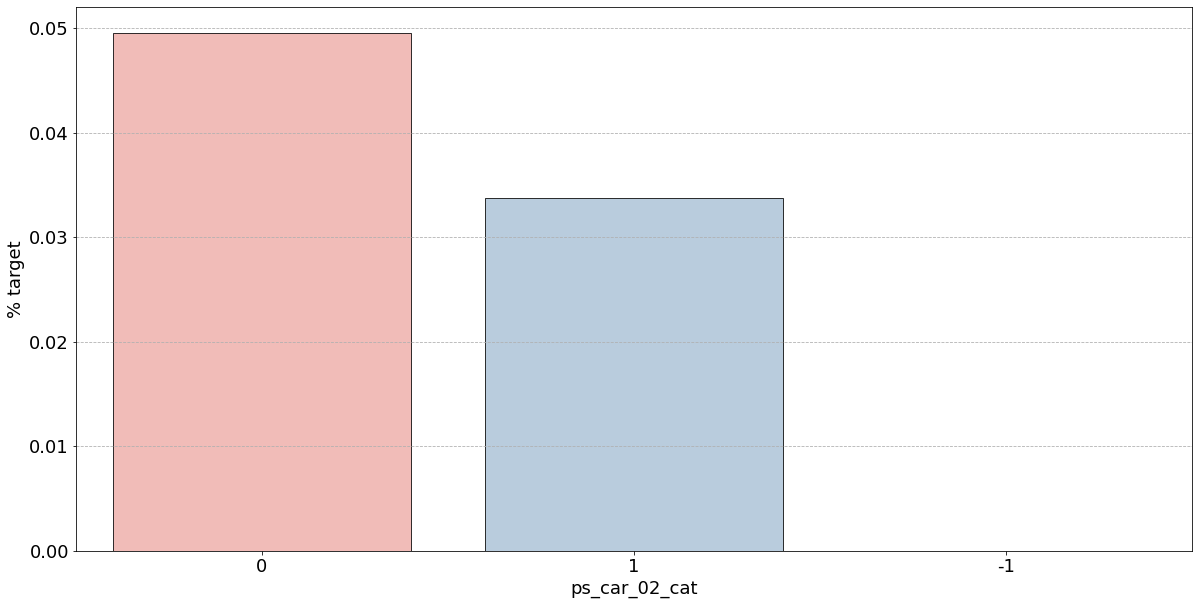
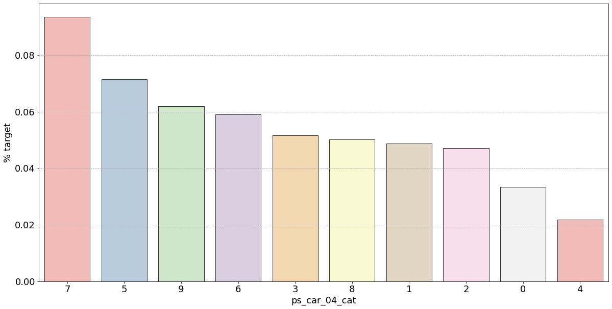
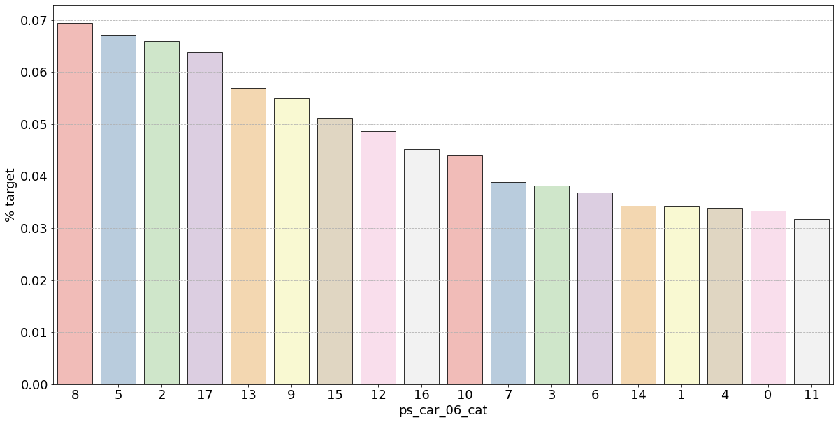
범주형 변수의 시각화

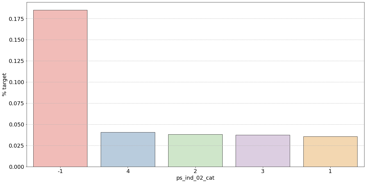
target값이 1인 범주형 변수들(고객들)의 특성을 시각화를 통해 비율 파악

Nominal = meta[(meta["level"] == 'nominal') & (meta["keep"])].index


# 변수별로 반복문을 돌려서 barplot을 그린다.
for f in Nominal:
    plt.figure()
    fig, ax = plt.subplots(figsize=(20,10))
    ax.grid(axis = "y", linestyle='--')
    
    # 변수 별 target=1의 비율 계산
    cat_perc = df_train[[f, 'target']].groupby([f],as_index=False).mean()
    cat_perc.sort_values(by='target', ascending=False, inplace=True)
    
    # 위에서 계산해준 비율을 통해 target = 1의 데이터 중 어떤 유니크값의 비율이 높은지 확인할 수 있음
    # target 평균을 내림차순으로 정렬하여 막대그래프 그리기
    sns.barplot(ax=ax, x=f, y='target',palette = "Pastel1", edgecolor='black', linewidth=0.8, data=cat_perc, order=cat_perc[f], )
    plt.ylabel('% target', fontsize=18)
    plt.xlabel(f, fontsize=18)
    plt.tick_params(axis='both', which='major', labelsize=18)
    plt.show();

< Figure size 432x288 with 0 Axes >

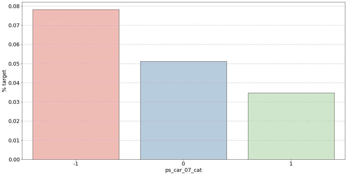
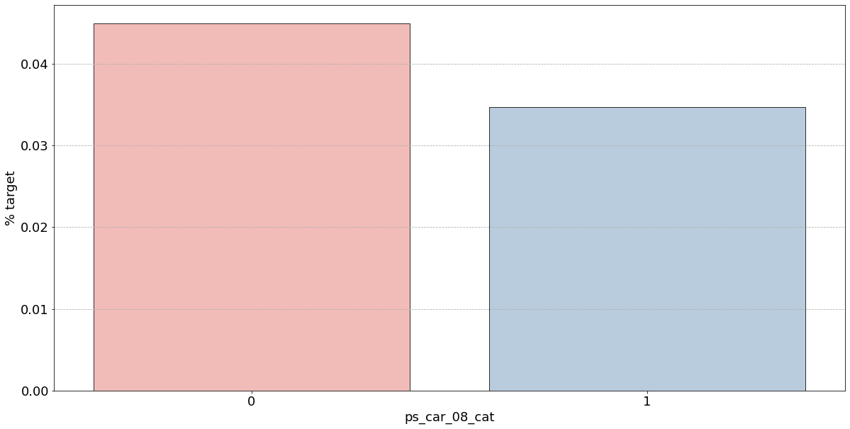
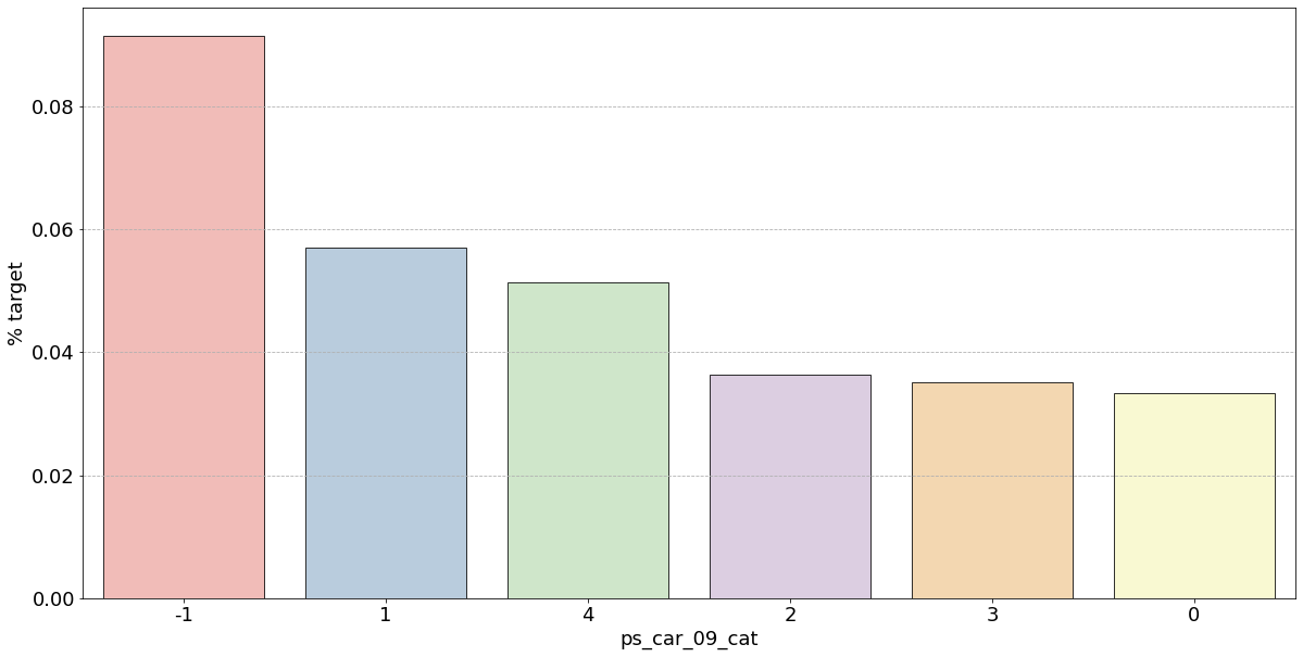
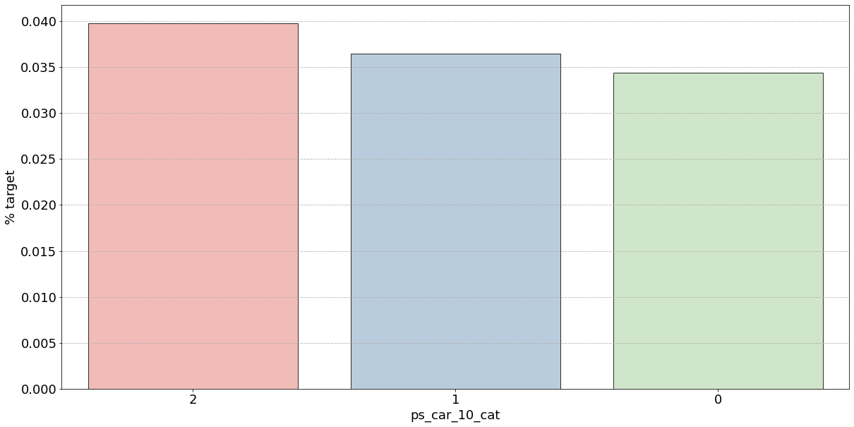
결측값은 모드로 대체하는 대신 별도의 범주 값으로 유지하는 것이 좋음
결측값을 가진 고객은 보험금 청구를 요청할 확률이 훨씬 높은(경우에 따라 훨씬 낮은) 것으로 보임
시각화한 barplot만 보면, 단순 비율로만 계산하고 count 값은 고려X이며 결측치가 많은 것은 대체해줬으므로 -1 count는 작은 것 밖에 안남아, 잘못된 인사이트를 얻을 수 있음

cf] 범주형 변수의 countplot이나 barplot을 그릴 때 groupby(hue를 지정)하여 살피면 어떤 feature을 만들 수 있을지 생각해볼 수 있음 → 더 다양한 인사이트 가질 수 있음

범주형 변수에 대한 결과
1. ps_ind_02_cat: -1(결측치)의 경우 target = 1의 데이터가 40%, 나머지는 10% 정도
  ✴️ 높다고 좋은게 아님!!
  ▪️ target 비율이므로 50%에 가까울수록 애매한 unique 값임
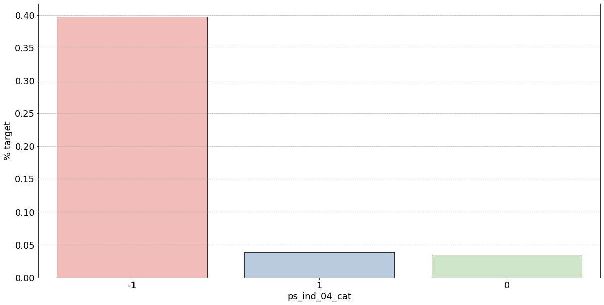
  ▪️ 차라리 10%인 나머지 unique 값들이 보험 청구를 안할 확률이 높다는 뜻으로 오히려 확실한 정보
2. ps_ind_04_cat: -1(결측치)가 65% 정도로 target = 1의 값을 가짐. 보험 청구할 확률이 높아보임
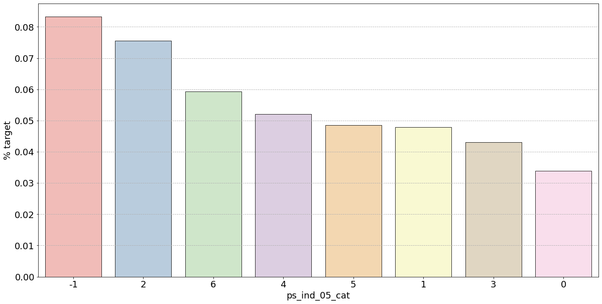
3. ps_ind_05_cat: unique 값 마다 차이가 있지만 눈에 띄지 X
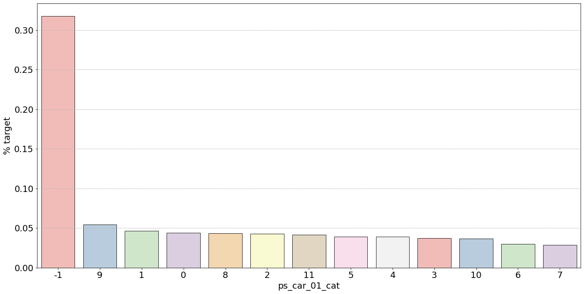
4. ps_car_01_cat: -1(결측치)가 거의 50%에 가까우므로 애매하고 나머지 값은 다 보험을 청구하지 않을 확률이 높아보임
5. ps_car_02_cat: -1(결측치)가 0%이므로 보험을 절대 청구하지 않을 것으로 보임

Interval 변수의 시각화(연속형)

구간 변수 간의 상관 관계를 확인
heatmap는 변수 간의 상관 관계를 시각화하는 좋은 방법
Seaborn의 diverging_palette() 클래스를 사용해서 양 끝 값들이 나뉘는 데이터에 대해 커스터마이징한 컬러맵을 만들 수 있음
- as_cmap=True 를 사용해서 생성한 팔레트를 seaborn이나 matplotlib에서 바로 쓸 수 있는 컬러맵 객체로도 받아오기도 가능
corr() : 각 열 간의 상관 계수를 반환하는 메서드

def corr_heatmap(Interval):
    correlations = df_train[Interval].corr()
    # corr() : 각 열 간의 상관 계수를 반환하는 메서드

    # Create color map ranging between two colors
    cmap = sns.diverging_palette(220, 10, as_cmap=True)

    fig, ax = plt.subplots(figsize=(10,10))
    sns.heatmap(correlations, cmap=cmap, vmax=1.0, center=0, fmt='.2f',
                square=True, linewidths=.5, annot=True, cbar_kws={"shrink": .75})
    plt.show();
    
Interval = meta[(meta["role"] == "target") | (meta["level"] == 'interval') & (meta["keep"])].index
corr_heatmap(Interval)

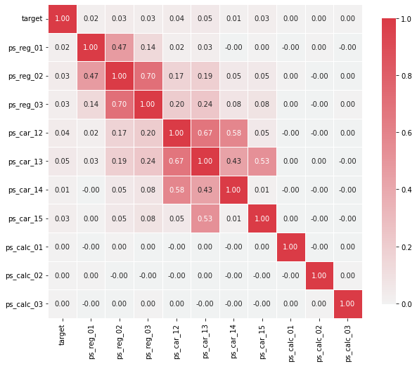
몇개의 변수들은 강한 상관관계를 보임
- ps_reg_02 & ps_reg_03 (0.7)
- ps_car_12 & ps_car_13 (0.67)
- ps_car_12 & ps_car_14 (0.58)
- ps_car_13 & ps_car_15 (0.67)
살펴본 강한 상관관계를 가지는 변수들에 대해 추가로 시각화를 진행
pairplot을 사용하여 변수 사이의 관계 시각화
heatmap에는 상관관계가 있는 변수의 수가 제한돼있으므로 각 변수를 개별적으로 살펴보자
- 프로세스 속도를 높이기 위해 train data sample 채취

s = train.sample(frac=0.1)

✳️ ps_reg_02 & ps_reg_03

sns.lmplot(x='ps_reg_02', y='ps_reg_03', data=df_train, hue='target', palette='Set1', scatter_kws={'alpha':0.3})
plt.show()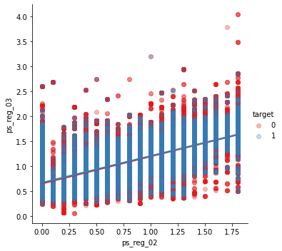

plot을 보면 두 개의 변수가 선형관계를 이루는 것을 확인할 수 있음
회귀선이 겹치거나 비슷한 모습
색상 매개변수로 인해 target = 0, 1의 회귀선이 동일함을 알 수 있음

✳️ ps_car_12 & ps_car_13

sns.lmplot(x='ps_car_12', y='ps_car_13', data=df_train, hue='target', palette='Set1', scatter_kws={'alpha':0.3})
plt.show()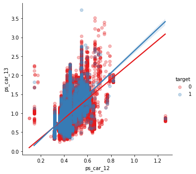

✳️ ps_car_12 & ps_car_14

sns.lmplot(x='ps_car_12', y='ps_car_14', data=df_train, hue='target', palette='Set1', scatter_kws={'alpha':0.3})
plt.show()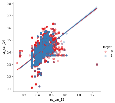

✳️ ps_car_13 & ps_car_15

sns.lmplot(x='ps_car_15', y='ps_car_13', data=df_train, hue='target', palette='Set1', scatter_kws={'alpha':0.3})
plt.show()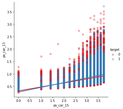

변수에 대한 PCA(주성분 분석)을 수행하여 치수를 줄일 수 있음
- 상관 변수의 수가 적으므로 모델이 heavy-lifting을 하도록 하자

Ordinal 변수의 시각화

Ordinal = meta[(meta["role"] == "target") | (meta["level"] == 'ordinal') & (meta["keep"])].index
corr_heatmap(Ordinal)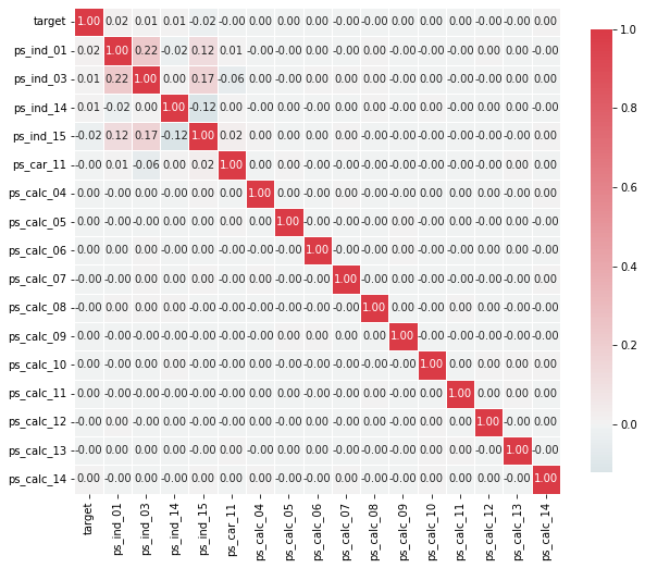

heatmap으로 상관관계 파악
순서형 변수의 경우 변수간에 큰 상관관계를 보이지 않음
- target 값을 grouping하면 분포가 어떻게 형성되는지 확인 가능

🔶Feature Engineering

Dummy 변수 생성

범주형 변수는 순서나 크기 나타내지 X
- category 2 ≠ (category 1) *2
이러한 문제해결을 위해 dummy 변수 활용
- 원래 변수의 범주에 대해 생성된 다른 dummy 변수에서 파생 가능 -> 첫번째 dummy 변수 삭제
unique 값을 갖는 범주형 변수가 아닌 나머지 변수들은 one-hot encoding 으로 dummy화
범주형 변수에 순서도 부여하지 않고, unique 값도 많지 않아 차원이 많이 늘어나지 X

v = meta[(meta["level"] == 'nominal') & (meta["keep"])].index
print('Before dummification we have {} variables in train'.format(df_train.shape[1]))
df_train = pd.get_dummies(df_train, columns=v, drop_first=True)
print('After dummification we have {} variables in train'.format(df_train.shape[1]))

Before dummification we have 57 variables in train
After dummification we have 109 variables in train

52개의 변수 증가

interaction 변수 생성

v = meta[(meta.level == 'interval') & (meta.keep)].index
poly = PolynomialFeatures(degree=2, interaction_only=False, include_bias=False)
interactions = pd.DataFrame(data=poly.fit_transform(df_train[v]), columns=poly.get_feature_names_out(v))
interactions.drop(v, axis=1, inplace=True)  # interactions 데이터프레임에서 기존 변수 삭제

# 새로 만든 변수들을 기존 데이터에 concat 시켜줌
print('Before creating interactions we have {} variables in train'.format(train.shape[1]))
train = pd.concat([df_train, interactions], axis=1)
print('After creating interactions we have {} variables in train'.format(train.shape[1]))

Before creating interactions we have 59 variables in train
After creating interactions we have 164 variables in train

train 데이터에 interaction 변수 추가
get_feature_names_out() 메서드로 열 이름을 새 변수에 할당 가능

🔶Feature 선택

분산이 낮거나 0인 feature 제거

Variance Threshold(분산임계값) : feature을 제거할 수 있는 sklearn의 방법
- 분산이 0인 형상 제거
- 이전 단계에서 zero-variance 변수 없었음
- 분산이 1% 미만인 feature 제거하면 31개의 변수 제거됨

selector = VarianceThreshold(threshold=.01)
selector.fit(df_train.drop(['id', 'target'], axis=1)) # Fit to train without id and target variables

f = np.vectorize(lambda x : not x) # Function to toggle boolean array elements

v = df_train.drop(['id', 'target'], axis=1).columns[f(selector.get_support())]
print('{} variables have too low variance.'.format(len(v)))
print('These variables are {}'.format(list(v)))

26 variables have too low variance.
These variables are ['ps_ind_10_bin', 'ps_ind_11_bin', 'ps_ind_12_bin', 'ps_ind_13_bin', 'ps_car_12', 'ps_car_14', 'ps_car_11_cat_te', 'ps_ind_05_cat_2', 'ps_ind_05_cat_5', 'ps_car_01_cat_0', 'ps_car_01_cat_1', 'ps_car_01_cat_2', 'ps_car_04_cat_3', 'ps_car_04_cat_4', 'ps_car_04_cat_5', 'ps_car_04_cat_6', 'ps_car_04_cat_7', 'ps_car_06_cat_2', 'ps_car_06_cat_5', 'ps_car_06_cat_8', 'ps_car_06_cat_12', 'ps_car_06_cat_16', 'ps_car_06_cat_17', 'ps_car_09_cat_4', 'ps_car_10_cat_1', 'ps_car_10_cat_2']

🔶Feature scaling

scaler = StandardScaler()
scaler.fit_transform(train.drop(['target'], axis=1))

박신영

기술블로그

index	id	ps_ind_01	ps_ind_02_cat	ps_ind_03	ps_ind_04_cat	ps_ind_06_bin	ps_ind_07_bin	ps_ind_08_bin	ps_ind_15	ps_ind_16_bin	ps_ind_17_bin	ps_ind_18_bin
0	7	2	2	5	1	0	1	0	11	0	1	0
1	9	1	1	7	0	0	0	1	3	0	0	1
2	13	5	4	9	1	0	0	1	12	1	0	0
3	16	0	1	2	0	1	0	0	8	1	0	0
4	17	0	2	0	1	1	0	0	9	1	0	0

index	id	ps_ind_01	ps_ind_02_cat	ps_ind_03	ps_ind_04_cat	ps_ind_06_bin	ps_ind_08_bin	ps_ind_09_bin	ps_ind_15	ps_ind_16_bin
595207	1488013	3	1	10	0	0	0	1	13	1
595208	1488016	5	1	3	0	0	0	1	6	1
595209	1488017	1	1	10	0	1	0	0	12	1
595210	1488021	5	2	3	1	0	1	0	12	1
595211	1488027	0	1	8	0	1	0	0	7	1

index	id	ps_ind_01	ps_ind_02_cat	ps_ind_03	ps_ind_04_cat	ps_ind_06_bin	ps_ind_07_bin	ps_ind_08_bin	ps_ind_15	ps_ind_16_bin	ps_ind_17_bin	ps_ind_18_bin
0	7	2	2	5	1	0	1	0	11	0	1	0
1	9	1	1	7	0	0	0	1	3	0	0	1
2	13	5	4	9	1	0	0	1	12	1	0	0
3	16	0	1	2	0	1	0	0	8	1	0	0
4	17	0	2	0	1	1	0	0	9	1	0	0