Numeriacal Differention
Deleting the terms involving ξ(x) gives
f′(x)≈hf(x0+h)−f(x0).
One difficulty with this formula is that we have no information about Dxf′′(ξ(x)), so the truncation error cannot be estimated. When x is x0, however, the coefficient of Dxf′′(ξ(x) ) is 0 , and the formula simplifies to
f′(x0)=hf(x0+h)−f(x0)−2hf′′(ξ).
For small values of h, the difference quotient [f(x0+h)−f(x0)]/h can be used to approximate f′(x0) with an error bounded by M∣h∣/2, where M is a bound on ∣f′′(x)∣ for x between x0 and x0+h. This formula is known as the forward-difference formula if h>0 (see Figure 4.1) and the backward-difference formula if h<0.
Example
Use the forward-difference formula to approximate the derivative of f(x)=lnx at x0=1.8 using h=0.1,h=0.05, and h=0.01, and determine bounds for the approximation errors.
f′(x0)=2h1[−3f(x0)+4f(x0+h)−f(x0+2h)]+3h2f(3)(ξ0),
where ξ0 lies between x0 and x0+2h.
f′(x0)=2h1[f(x0+h)−f(x0−h)]−6h2f(3)(ξ1)
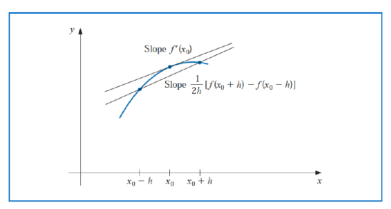
The methods presented in Eqs. (4.4) and (4.5) are called three-point formulas (even though the third point f(x0) does not appear in Eq. (4.5)). Similarly, there are five-point formulas that involve evaluating the function at two additional points. The error term for these formulas is O(h4). One common five-point formula is used to determine approximations for the derivative at the midpoint.
- f′(x0)=12h1[f(x0−2h)−8f(x0−h)+8f(x0+h)−f(x0+2h)]+30h4f(5)(ξ),
where ξ lies between x0−2h and x0+2h.
f′(x0)=12h1[−25f(x0)+48f(x0+h)−36f(x0+2h)+16f(x0+3h)−3f(x0+4h)]+5h4f(5)(ξ),
where ξ lies between x0 and x0+4h.
Left-endpoint approximations are found using this formula with h>0 and right-endpoint approximations with h<0. The five-point endpoint formula is particularly useful for the clamped cubic spline interpolation of Section 3.5.
Example 2
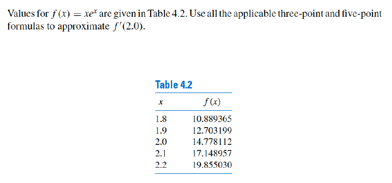
Values for f(x)=xex are given in Table 4.2. Use all the applicable three-point and five-point formulas to approximate f′(2.0).
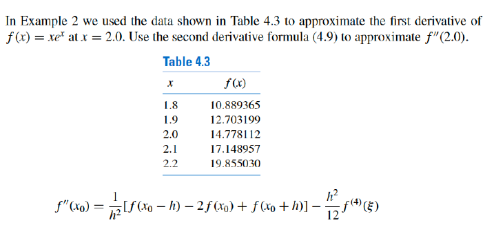
f′′(x0)=h21[f(x0−h)−2f(x0)+f(x0+h)]−12h2f(4)(ξ),
for some ξ, where x0−h<ξ<x0+h.
If f(4) is continuous on [x0−h,x0+h] it is also bounded, and the approximation is O(h2).
Example3
Round-Off Error Instability
It is particularly important to pay attention to round-off error when approximating derivatives. To illustrate the situation, let us examine the three-point midpoint formula Eq. (4.5),
f′(x0)=2h1[f(x0+h)−f(x0−h)]−6h2f(3)(ξ1),
more closely. Suppose that in evaluating f(x0+h) and f(x0−h) we encounter round-off errors e(x0+h) and e(x0−h). Then our computations actually use the values f~(x0+h) and f~(x0−h), which are related to the true values f(x0+h) and f(x0−h) by
f(x0+h)=f~(x0+h)+e(x0+h) and f(x0−h)=f~(x0−h)+e(x0−h). 