[Project] Video Game 기획 프로젝트

Kyung Jae, Cheong·2022년 11월 5일

개인프로젝트 코드스테이츠

개인프로젝트

목록 보기

1/17

코드스테이츠 AI 부트캠프 Section1에서 다음 분기에 어떤 게임을 설계해야 할까? 라는 공통주제로 실시한 Data Science 개인프로젝트 내용 정리 및 회고.

Github Repository 바로가기 : Project-GamePlanning (클릭)

어떤 게임을 설계해야할까?

Tech Stack

00. 프로젝트 개요

상황 가정 & 필수 포함 요소

게임 회사의 데이터 팀에 합류했다고 가정
- 다음 분기에 어떤 게임을 설계해야 할까 라는 고민을 해결하는 것이 프로젝트 목표
발표를 듣는 사람은 비데이터 직군이라 가정
- 최대한 배경지식이 없는 사람들도 이해할 수 있도록 노력하는 것이 부가적인 목표
필수 포함 요소
- 지역에 따라서 선호하는 게임 장르가 다를까
- 연도별 게임의 트렌드가 있을까
- 출고량이 높은 게임에 대한 분석 및 시각화 프로세스

프로젝트 목차

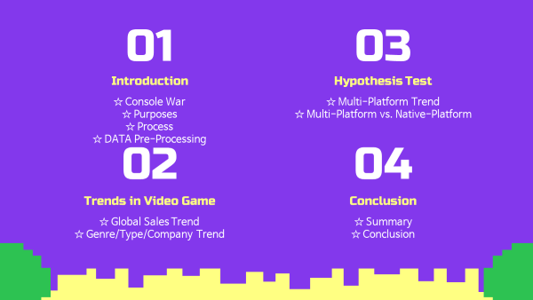
Introduction 서론
- Console War(1977~) 배경지식
- Purposes 프로젝트 목표
- Process 프로젝트 진행 절차
Data 데이터
- Data Pre-processing 데이터 전처리
- Feature Engineering 특성 조합
Trends in Video Game 트렌드 분석
- Global Sales Trend 글로벌 트렌드
- Genre Trend 장르 트렌드
- Platform Type Trend 게임플랫폼 타입 트렌드
- Platform Company Trend 플랫폼 기업 트렌드
Hypothesis Test 가설 검정
- Multi-Platform vs. Native-Platform 멀티플랫폼과 단일플랫폼
Conclusion 결론
- Summary 요약
- Conclusion 결론 및 인사이트 도출
- Retrospective 회고

01. Introduction 서론

1-1. Console War(1977~) 배경지식 - 콘솔전쟁

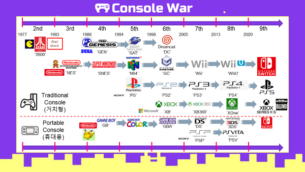
2세대 (1977~1983) - 아타리 독점
- Atari ATARI 2600
  - 플랫폼 형태의 최초 콘솔 게임기
  - 1983년 Atari Shock에 의해 몰락
  - 대표작 : PACKMAN(1980)
3세대 (1983~1988) - 닌텐도 독점
- Nintendo NES(패미컴)
  - 닌텐도의 게임기 시장 진출 및 독점
  - 대표작 : MARIO BROS(1983)
4세대 (1988~1994) - 전쟁의 서막
- Nintendo SNES(슈퍼패미컴) GAMEBOY(게임보이)
  - 닌텐도의 휴대용 게임기 시장 진출
  - 대표작 : POKEMON(1996)
- SEGA GENESIS(메가드라이브)
  - 세가의 참전
  - 대표작 : SONIC THE HEDGHOG(1991)
5세대 (1994~1998) - 삼국지 시대 개막
- Nintendo N64(닌텐도64)
- SEGA SATURN(새턴)
- SONY PlayStation(플레이스테이션)
  - 소니의 참전
  - 일본 게임사의 삼국지 형성
6세대 (1998~2005) - SONY 몰락, Microsoft 참전
- Nintendo GAMECUBE(게임큐브) GBA(게임보이어드밴스)
- SONY PS2(플스2)
- Microsoft XBOX(엑스박스)
  - 마이크로소프트의 콘솔게임시장 진출
  - 현재까지 이어져오는 3강구도가 형성됨
7세대 (2005~2013) - 비디오 콘솔게임시장의 최고 전성기
- Nintendo Wii(닌텐도 위) NDS(닌텐도DS)
- SONY PS3(플스3) PSP(플스포터블)
  - SONY의 휴대용 게임기 시장 진출
- Microsoft XBOX360(엑스박스360)
8세대 (2013~2020) - 비디오 콘솔게임 시장의 쇠퇴
- Nintendo Wii(닌텐도 위) NDS(닌텐도DS)
- SONY PS4(플스4) PSP(플스포터블)
  - SONY의 휴대용 게임기 시장 진출
- Microsoft XBOX360(엑스박스360)
9세대 (2020~현재) - 현재 3강구도
- Nintendo Nintendo SWITCH(닌텐도 스위치)
- SONY PS5(플레이스테이션5)
- Microsoft XBOX SERIES X|S(엑스박스 시리즈 X|S)

1-2. Purposes 프로젝트 목표

Genre : 어떤 장르의 게임을 선호하는가?
Platform Type : 거치형 콘솔, 휴대용 콘솔, PC 중 어떤 type을 선호하는가?
Platform Company : 어떤 기업의 플랫폼을 선호하는가?
- Multi-Platform으로 개발하는 것이 효과적일까?

1-3. Process 프로젝트 진행 절차

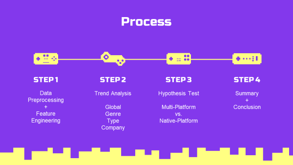
데이터
- Data Preprocessing (데이터 전처리)
- Feature Engineering (특성 조합)
트렌드 분석
- Global 트렌드
- 장르 트렌드
- 플랫폼 타입 트렌드
- 플랫폼 기업 트렌드
가설 검정
- 멀티플랫폼 vs 단일플랫폼 T-test
- 지역별 T-test
결론
- 요약, 결론

02. Data 데이터

2-1. Data Preprocessing 데이터 전처리

STEP0. Data Import 데이터 불러오기

# csv 파일 불러오기
df = pd.read_csv('vgames2.csv')
# 첫 column은 의미 없는 index Data이므로 제외
df1 = df.iloc[:,1:]
display(df1.head())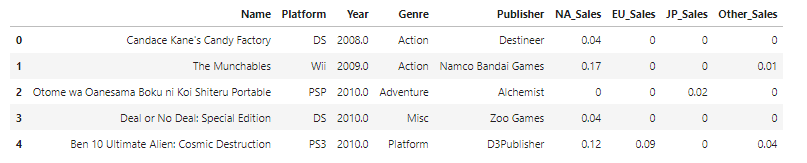

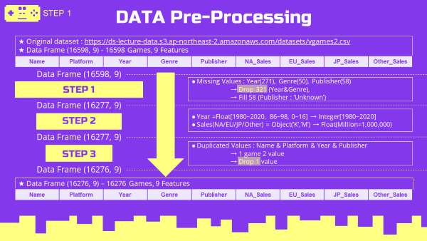
STEP1. 결측치 처리

결측치 확인

#결측치 확인
df1.isnull().sum()
#output
'''
Name             0
Platform         0
Year           271
Genre           50
Publisher       58
NA_Sales         0
EU_Sales         0
JP_Sales         0
Other_Sales      0
dtype: int64
'''
#원본데이터 shape
df1.shape
#output
'''
(16598, 9)
'''

Year, Genre는 중요한 factor, 다른 특성에서 대체할 방법이 없음 - DROP

#결측치 row 쿼리 후 drop
df_year_null = df1[df1.Year.isnull()|df.Genre.isnull()]
df1_drop = df1.drop(index=df_year_null.index).reset_index(drop=True)
#shape 확인
df1_drop.shape
#output
'''
(16277, 9)
'''
#제거된 row 수
df1.shape[0]-df1_drop.shape[0]
#output
'''
321
'''

Publisher는 데이터 분석에서 참고용 자료로 쓸예정, Unknown 으로 대체

#fillna함수 이용
df2 = df1_drop.copy()
df2.Publisher = df2.Publisher.fillna('Unknown')

제거 후 결측치 확인

#결측치 확인
df2.isnull().sum()
#output
'''
Name           0
Platform       0
Year           0
Genre          0
Publisher      0
NA_Sales       0
EU_Sales       0
JP_Sales       0
Other_Sales    0
dtype: int64
'''
#결측치 처리후 shape
df2.shape
#output
'''
(16277, 9)
'''

STEP2. 오류 데이터 확인, 대체

column 순서대로 확인 진행

Platform column 확인

#Platform column
df2.Platform.unique()
#output
'''
array(['DS', 'Wii', 'PSP', 'PS3', 'PC', 'PS', 'GBA', 'PS4', 'PS2', 'XB',
     'X360', 'GC', '3DS', '2600', 'SAT', 'GB', 'NES', 'DC', 'N64',
     'XOne', 'SNES', 'WiiU', 'PSV', 'GEN', 'SCD', 'WS', 'NG', 'TG16',
     '3DO', 'GG', 'PCFX'], dtype=object)
'''

사전 조사 결과에 따라 Platform column의 표기 오류는 없었음.

Year column 확인

#Year column
df2.Year.unique()
#ouput
'''
array([2.008e+03, 2.009e+03, 2.010e+03, 2.005e+03, 2.011e+03, 2.007e+03,
     2.001e+03, 2.003e+03, 2.006e+03, 2.014e+03, 2.015e+03, 2.002e+03,
     1.997e+03, 2.013e+03, 1.996e+03, 2.004e+03, 2.000e+03, 1.984e+03,
     1.998e+03, 2.016e+03, 1.985e+03, 1.999e+03, 9.000e+00, 9.700e+01,
     1.995e+03, 1.993e+03, 2.012e+03, 1.987e+03, 1.982e+03, 1.100e+01,
     1.994e+03, 1.990e+03, 1.500e+01, 1.992e+03, 1.991e+03, 1.983e+03,
     1.988e+03, 1.981e+03, 3.000e+00, 1.989e+03, 9.600e+01, 6.000e+00,
     8.000e+00, 1.986e+03, 1.000e+00, 5.000e+00, 4.000e+00, 1.000e+01,
     9.800e+01, 7.000e+00, 1.600e+01, 8.600e+01, 1.400e+01, 9.500e+01,
     2.017e+03, 1.980e+03, 2.020e+03, 2.000e+00, 1.300e+01, 0.000e+00,
     1.200e+01, 9.400e+01])
'''
#Year Series 정의 후 타입 integer로 변경
Year_series = df2.Year.astype(int)
Year_series.unique()
#output
'''
array([2008, 2009, 2010, 2005, 2011, 2007, 2001, 2003, 2006, 2014, 2015,
     2002, 1997, 2013, 1996, 2004, 2000, 1984, 1998, 2016, 1985, 1999,
        9,   97, 1995, 1993, 2012, 1987, 1982,   11, 1994, 1990,   15,
     1992, 1991, 1983, 1988, 1981,    3, 1989,   96,    6,    8, 1986,
        1,    5,    4,   10,   98,    7,   16,   86,   14,   95, 2017,
     1980, 2020,    2,   13,    0,   12,   94])
'''

Year 표기형태 통일을 위해 수정 필요

# 함수정의
def year(y):
  if (y>=0) and (y<22):
      y = y+2000
  elif (y>=22) and (y<1000):
      y = y+1900
  else:
      y = y
  return y
# apply 후 확인
Year_fix = Year_series.apply(year)
Year_fix.unique()
#output
'''
array([2008, 2009, 2010, 2005, 2011, 2007, 2001, 2003, 2006, 2014, 2015,
     2002, 1997, 2013, 1996, 2004, 2000, 1984, 1998, 2016, 1985, 1999,
     1995, 1993, 2012, 1987, 1982, 1994, 1990, 1992, 1991, 1983, 1988,
     1981, 1989, 1986, 2017, 1980, 2020], dtype=int64)
'''
# 수정결과 덮어쓰기
df3 = df2.copy()
df3.Year = Year_fix
df3.Year.unique()
#output
'''
array([2008, 2009, 2010, 2005, 2011, 2007, 2001, 2003, 2006, 2014, 2015,
     2002, 1997, 2013, 1996, 2004, 2000, 1984, 1998, 2016, 1985, 1999,
     1995, 1993, 2012, 1987, 1982, 1994, 1990, 1992, 1991, 1983, 1988,
     1981, 1989, 1986, 2017, 1980, 2020], dtype=int64)
'''

Genre column 확인

#Genre column
df3.Genre.unique()
#output
'''
array(['Action', 'Adventure', 'Misc', 'Platform', 'Sports', 'Simulation',
     'Racing', 'Role-Playing', 'Puzzle', 'Strategy', 'Fighting',
     'Shooter'], dtype=object)
'''

Genre column 이상없음

Sales column 확인

#Sales column
df3.iloc[:,-4:].dtypes
#output
'''
NA_Sales       object
EU_Sales       object
JP_Sales       object
Other_Sales    object
dtype: object
'''

object인 것으로 보아 숫자가 아닌 데이터가 섞여있을 가능성이 커보임
일단 NorthAmerica 알파벳이 있는 열을 확인해봄

df3_NA_err = df3[df3.NA_Sales.str.contains('[a-zA-Z]')]
df3_NA_err.head()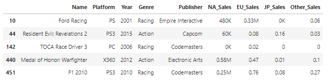

K와 M이 보임.

K는 1,000 M은 1,000,000

K,M이 안붙어있는 데이터의 단위가 M인것으로 확인함

단위를 M으로 통일시키도록 하겠음

#함수정의
def scalefix(s):
  if s.endswith('K'):
      s = s.replace('K','')
      s = float(s)*0.001
  elif s.endswith('M'):
      s = s.replace('M','')
  return s
#NA_Sales에 적용해보기
df3_fix_test = df3_NA_err.NA_Sales.apply(scalefix)
df3_fix_test.head()
#output
'''
10     0.48
44     0.06
142     0.0
440    0.58
451    0.25
Name: NA_Sales, dtype: object
'''
#모든 Sales column에 적용
df3_Sales = df3.iloc[:,-4:]
df3_Sales_fix = df3_Sales.applymap(scalefix)
df3_Sales_fix_f = df3_Sales_fix.astype(float)
#수정사항 덮어쓰기
df4 = df3.copy()
df4.iloc[:,-4:] = df3_Sales_fix_f
display(df4.dtypes)
#output
Name            object
Platform        object
Year             int64
Genre           object
Publisher       object
NA_Sales       float64
EU_Sales       float64
JP_Sales       float64
Other_Sales    float64
dtype: object
#.describe() 로 확인 (max값 확인)
display(df4.describe())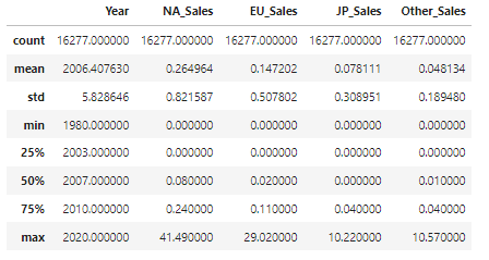

STEP3. 중복치 확인, 제거

Name, Platform, Year, Publisher가 같다면 같은 게임으로 취급

df4[df4.duplicated(subset=['Name','Platform','Year','Publisher'],keep=False)]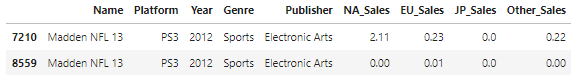

index 8559의 데이터는 오류인 것으로 판단, 제거

#index 8559 제거
df5 = df4.drop(index=8559).reset_index(drop=True)
#중복치 제거 후 shape
df5.shape
#output
'''
(16276, 9)
'''

STEP4. 전처리 데이터 저장

df5.to_csv('vgames_pre.csv',index=False)

2-2. Feature Engineering 특성 조합

STEP0. Data Import 데이터 불러오기

fe = pd.read_csv('vgames_pre.csv')
fe.head()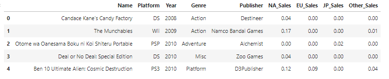

#데이터 shape
fe.shape
#output
'''
(16276, 9)
'''

STEP1. Global Sales feature 생성

fe1 = fe.copy()
fe1['Global_Sales'] = fe1.NA_Sales+fe1.EU_Sales+fe1.JP_Sales+fe1.Other_Sales
fe1.describe()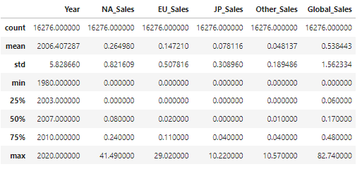

#데이터 shape
fe1.shape
#output
'''
(16276, 10)
'''

STEP2. Platform type feature 생성

Platform column value 확인

#Platform column
print('platform 수 : {}'.format(len(fe1.Platform.unique())))
fe1.Platform.unique()
#output
'''
platform 수 : 31
array(['DS', 'Wii', 'PSP', 'PS3', 'PC', 'PS', 'GBA', 'PS4', 'PS2', 'XB',
       'X360', 'GC', '3DS', '2600', 'SAT', 'GB', 'NES', 'DC', 'N64',
       'XOne', 'SNES', 'WiiU', 'PSV', 'GEN', 'SCD', 'WS', 'NG', 'TG16',
       '3DO', 'GG', 'PCFX'], dtype=object)
'''

사전조사에 의한 Platform 타입별 분류

Traditional = ['2600','NES','SNES','N64','GC','Wii','WiiU',
               'GEN','SAT','DC','PS','PS2','PS3','PS4',
               'XB','X360','XOne']
Portable = ['GB','GBA','DS','3DS','PSP','PSV']
PC = ['PC']

분류에 포함되지 않는 데이터 수 확인

#분류 미포함 쿼리
fe1_type = fe1[~fe1.Platform.isin(Traditional+Portable+PC)]
print('분류에 포함되지 않는 데이터 수: {}'.format(fe1_type.shape[0]))
#output
'''
분류에 포함되지 않는 데이터 수: 31
'''

전체 집단에비해 수가 매우 작으므로 제거

#drop
fe2 = fe1.copy()
fe2 = fe2.drop(index=fe1_type.index).reset_index(drop=True)
fe_type_check = fe2[~fe2.Platform.isin(Traditional+Portable+PC)]
print('제거 후 분류에 포함되지 않는 데이터 수: {}'.format(fe_type_check.shape[0]))
print('\nplatform 수 : {}'.format(len(fe2.Platform.unique())))
#output
'''
제거 후 분류에 포함되지 않는 데이터 수: 0

platform 수 : 24
'''
#platform목록 일치여부 확인
print(set(fe2.Platform.unique()) == set(Traditional+Portable+PC))
#output
'''
True
'''

platform type으로 반환시키는 함수 정의후 feature 추가

#platform type으로 반환시키는 함수 정의
def plat_type(p):
    if p in Traditional:
        p = 'Traditional'
    elif p in Portable:
        p = 'Portable'
    elif p in PC:
        p = 'PC'
    return p
#platform type column 생성
fe2_type = fe2.copy()
fe2_type['Platform_type'] = fe2_type.Platform.apply(plat_type)
#함수오류로 입력안된 값이 있는지를 확인
print(fe2_type.Platform_type.isnull().sum())
#output
'''
0
'''
display(fe2_type.head())

#데이터 shape
fe2_type.shape
#output
'''
(16245, 11)
'''

STEP3. Platform company feature 생성

사전조사에 의한 Platform company 분류

Atari = ['2600']
Nintendo = ['NES','SNES','N64','GC','Wii','WiiU','GB','GBA','DS','3DS']
Sega = ['GEN','SAT','DC']
Sony = ['PS','PS2','PS3','PS4','PSP','PSV']
Microsoft = ['XB','X360','XOne']
PC = ['PC']

platform 목록이 분류했던 목록과 일치하는지 확인

print(set(fe2_type.Platform.unique()) == set(Atari+Nintendo+Sega+Sony+Microsoft+PC))
#output
'''
True
'''

Platform company feature 생성

#platform company으로 반환시키는 함수 정의
def plat_company(p):
    if p in Atari:
        p = 'Atari'
    elif p in Nintendo:
        p = 'Nintendo'
    elif p in Sega:
        p = 'Sega'
    elif p in Sony:
        p = 'Sony'
    elif p in Microsoft:
        p = 'Microsoft'
    elif p in PC:
        p = 'PC'
    return p
#platform type column 생성
fe2_comp = fe2_type.copy()
fe2_comp['Platform_company'] = fe2_comp.Platform.apply(plat_company)
#함수오류로 입력안된 값이 있는지를 확인
print(fe2_comp.Platform_company.isnull().sum())
#output
'''
0
'''
display(fe2_comp.head())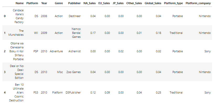

#데이터 shape
fe2_comp.shape
#output
'''
(16245, 12)
'''

STEP4. Generation feature 생성

사전조사에 의한 Generation 분류

gen2 = ['2600']
gen3 = ['NES']
gen4 = ['SNES','GEN','GB']
gen5 = ['N64','SAT','PS']
gen6 = ['GC','DC','PS2','XB','GBA']
gen7 = ['Wii','PS3','X360','DS','PSP']
gen8 = ['WiiU','PS4','XOne','3DS','PSV']
PC = ['PC']

Generation 분류가 platform 목록과 일치하는지 확인

print(set(fe2_comp.Platform.unique()) == set(gen2+gen3+gen4+gen5+gen6+gen7+gen8+PC))
#output
'''
True
'''

Generation feature 생성
- PC는 연도에 따라 기입 예정이라 np.nan으로 변환

#platform generation 반환 함수 정의
def plat_gen(p):
    if p in gen2:
        p = 2
    elif p in gen3:
        p = 3
    elif p in gen4:
        p = 4
    elif p in gen5:
        p = 5
    elif p in gen6:
        p = 6
    elif p in gen7:
        p = 7
    elif p in gen8:
        p = 8
    elif p in PC:
        p = np.nan
    return p
# Generation column 생성
fe2_gen = fe2_comp.copy()
fe2_gen['Generation']=fe2_gen.Platform.apply(plat_gen)
# 결측치 확인(PC와 일치여부)
print(fe2_gen.Generation.isnull().sum())
print(sum(fe2_gen.Platform=='PC'))
#output
'''
940
940
'''

PC game 연도별 분리 및 Generation 채우기

#세대별 분리
fe2_gen2 = fe2_gen.query('1977 < Year <= 1983')
fe2_gen3 = fe2_gen.query('1983 < Year <= 1988')
fe2_gen4 = fe2_gen.query('1988 < Year <= 1994')
fe2_gen5 = fe2_gen.query('1994 < Year <= 1998')
fe2_gen6 = fe2_gen.query('1998 < Year <= 2005')
fe2_gen7 = fe2_gen.query('2005 < Year <= 2013')
fe2_gen8 = fe2_gen.query('2013 < Year <= 2020')
#generation 채워넣기
fe2_f_gen2 = fe2_gen2.copy()
fe2_f_gen2.Generation = fe2_f_gen2.Generation.fillna('2')
fe2_f_gen3 = fe2_gen3.copy()
fe2_f_gen3.Generation = fe2_f_gen3.Generation.fillna('3')
fe2_f_gen4 = fe2_gen4.copy()
fe2_f_gen4.Generation = fe2_f_gen4.Generation.fillna('4')
fe2_f_gen5 = fe2_gen5.copy()
fe2_f_gen5.Generation = fe2_f_gen5.Generation.fillna('5')
fe2_f_gen6 = fe2_gen6.copy()
fe2_f_gen6.Generation = fe2_f_gen6.Generation.fillna('6')
fe2_f_gen7 = fe2_gen7.copy()
fe2_f_gen7.Generation = fe2_f_gen7.Generation.fillna('7')
fe2_f_gen8 = fe2_gen8.copy()
fe2_f_gen8.Generation = fe2_f_gen8.Generation.fillna('8')

분리한 Data병합

#분리한 Data를 합치고 타입을 int로 변환
fe2_f_gen = pd.concat([fe2_f_gen2,
						fe2_f_gen3,
                        fe2_f_gen4,
                        fe2_f_gen5,
                        fe2_f_gen6,
                        fe2_f_gen7,
                        fe2_f_gen8]).sort_index()
fe2_f_gen.Generation = fe2_f_gen.Generation.astype(int)
#데이터 확인
fe2_f_gen.info()
#output
'''
Int64Index: 16245 entries, 0 to 16244
Data columns (total 13 columns):
 #   Column            Non-Null Count  Dtype  
---  ------            --------------  -----  
 0   Name              16245 non-null  object 
 1   Platform          16245 non-null  object 
 2   Year              16245 non-null  int64  
 3   Genre             16245 non-null  object 
 4   Publisher         16245 non-null  object 
 5   NA_Sales          16245 non-null  float64
 6   EU_Sales          16245 non-null  float64
 7   JP_Sales          16245 non-null  float64
 8   Other_Sales       16245 non-null  float64
 9   Global_Sales      16245 non-null  float64
 10  Platform_type     16245 non-null  object 
 11  Platform_company  16245 non-null  object 
 12  Generation        16245 non-null  int32  
dtypes: float64(5), int32(1), int64(1), object(6)
memory usage: 1.7+ MB
'''

#데이터 shape
fe2_f_gen.shape
#output
'''
(16245, 13)
'''

STEP5. 멀티플랫폼 feature 생성

단일,멀티여부를 구분하는 column 생성을 위해 이름 기준으로 나눠줌

#데이터 분리
fe2_mono = fe2_f_gen[~fe2_f_gen.Name.duplicated(keep=False)]
fe2_multi = fe2_f_gen[fe2_f_gen.Name.duplicated(keep=False)]
#shape 확인
print(fe2_mono.shape)
print(fe2_multi.shape)
print(fe2_f_gen.shape)
fe2_f_gen.shape[0] == fe2_mono.shape[0]+fe2_multi.shape[0]
#output
'''
(8594, 13)
(7651, 13)
(16245, 13)
True
'''

멀티플랫폼 column 생성

#멀티플랫폼 지원여부 column 생성
fe2_mono2 = fe2_mono.copy()
fe2_multi2 = fe2_multi.copy()
fe2_mono2['Platform_Multi'] = 'Native'
fe2_multi2['Platform_Multi'] = 'Multi'
fe2_multi = pd.concat([fe2_mono2,fe2_multi2]).sort_index()
#shape 확인 
fe2_multi.shape
#output
'''
(16245, 14)
'''

STEP6. 최종 데이터 저장

column 순서 바꾸기

fe3 = fe2_multi.copy()
fe3 = fe3[['Name', 'Publisher', 'Year', 'Genre', 'Generation',
			'Platform', 'Platform_type', 'Platform_company', 'Platform_Multi', 
			'NA_Sales', 'EU_Sales', 'JP_Sales', 'Other_Sales', 'Global_Sales']]

최종 데이터 저장

fe3.to_csv('vgames_final.csv',index=False)

03. Trends in Video Game 트렌드 분석

시각화 패키지(라이브러리)

matplotlib.pyplot
seaborn
plotly

import matplotlib.pyplot as plt
plt.rcParams['font.family'] = 'Malgun Gothic'
plt.rcParams['axes.unicode_minus'] = False
import seaborn as sns
import plotly.express as plex
from plotly.subplots import make_subplots as plsub
import plotly.graph_objects as go

3-0. Data Import 데이터 불러오기

vgames = pd.read_csv('vgames_final.csv')
vgames.head()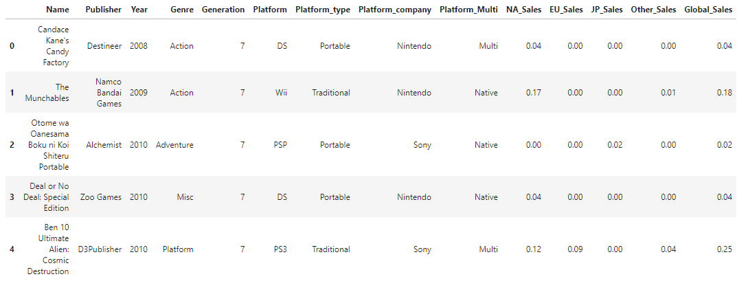

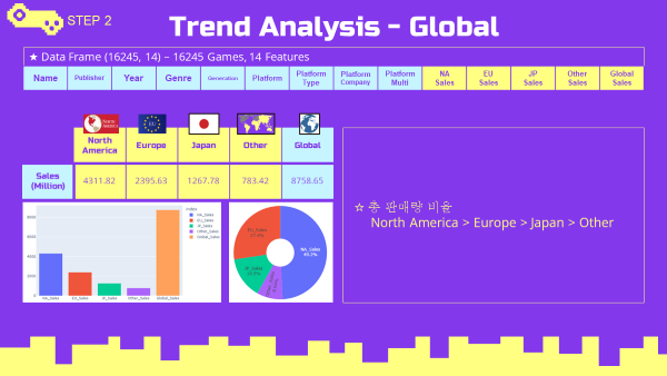
3-1. Global Sales Trend 전세계 판매량 트렌드 분석

글로벌 총 판매량

총 판매량은 북미, 유럽, 일본, 그외 지역 순으로 높게 나타남.
총 판매량 확인

Sales_list = ['NA_Sales','EU_Sales','JP_Sales','Other_Sales','Global_Sales']
df_global_sum = vgames[Sales_list].sum()
df_global_sum
#output
'''
NA_Sales        4311.82
EU_Sales        2395.63
JP_Sales        1267.78
Other_Sales      783.42
Global_Sales    8758.65
dtype: float64
'''

총 판매량 bar chart (plotly)

global_sum_bar = plex.bar(df_global_sum,color=df_global_sum.index)
global_sum_bar.show()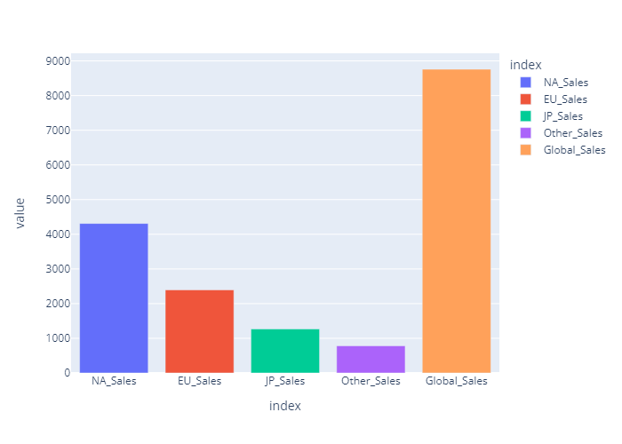

총 판매량 pie chart (plotly)

se_global_sum_pie = df_global_sum[:-1]
sum_index = se_global_sum_pie.index
sum_value = se_global_sum_pie.values
global_sum_pie = go.Figure(data=[go.Pie(labels=sum_index,
                                  values=sum_value,
                                  hole=.3,
                                  textinfo='label+percent')])
global_sum_pie.show()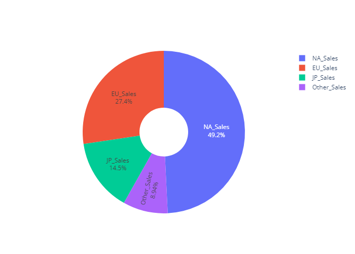

연도(세대)별 총 판매량

전반적으로 북미 지역에서의 매출 비율이 높게 나타남.
스마트폰 등장 시기인 2010년을 기점으로 전체적인 판매량이 하락하는 추세를 보임.
연도(세대)별 판매량 Grouping

df_year = vgames.groupby(['Year'],as_index=True)[Sales_list].sum()
df_gen = vgames.groupby(['Generation'],as_index=True)[Sales_list].sum()

연도별 판매량 line plot (matplotlib, seaborn)

plt.figure(figsize=(12,8))
sns.set_style('whitegrid')
sns.lineplot(data=df_year,markers=True,dashes=False)
plt.axvline(x=1980, color='gray',linestyle='--')
plt.axvline(x=1983, color='gray',linestyle='--')
plt.axvline(x=1988, color='gray',linestyle='--')
plt.axvline(x=1994, color='gray',linestyle='--')
plt.axvline(x=1998, color='gray',linestyle='--')
plt.axvline(x=2005, color='gray',linestyle='--')
plt.axvline(x=2013, color='gray',linestyle='--')
plt.axvline(x=2020, color='gray',linestyle='--')
plt.xlabel('')
plt.ylabel('Sales(Million)',fontsize=16)
plt.show()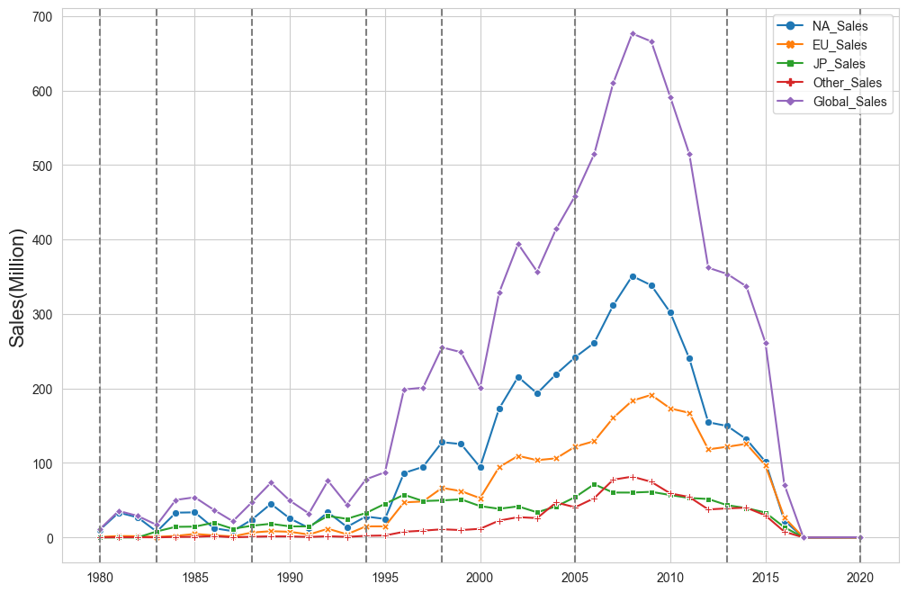

세대별 판매량 bar chart (plotly)

year_genre = plex.bar(data_frame=df_gen,title='Sales Trend(Global)',barmode='group')
year_genre.update_layout(yaxis_title='Sales(Million)')
year_genre.show()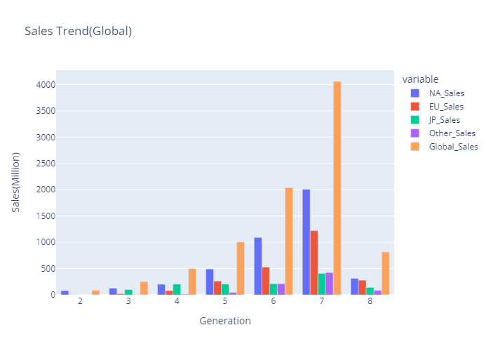

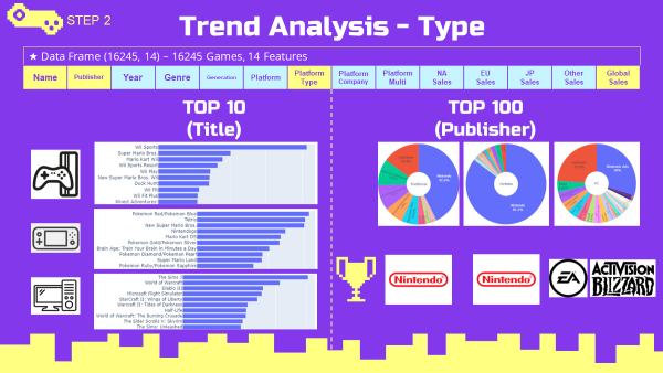
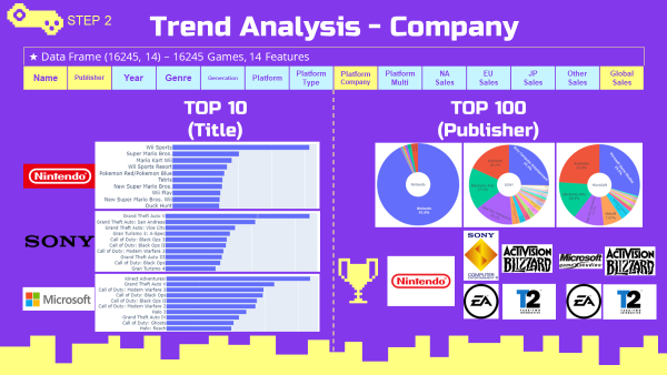
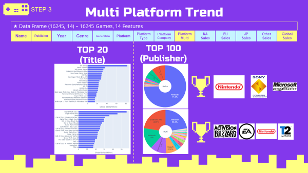
최고 매출 게임 및 개발사 분석

세계적으로 가장 많이 팔린 타이틀은 닌텐도의 Wii Sports.
100위권에는 닌텐도에서 개발한 게임들이 많은 비중을 차지함.
Top20, Top100 데이터

top20_global = vgames.sort_values(by='Global_Sales',ascending=False).head(20).reset_index(drop=True)
top100_global = vgames.sort_values(by='Global_Sales',ascending=False).head(100).reset_index(drop=True)

Top20 타이틀 bar chart (plotly)

global_top20_name = plex.bar(x=top20_global.Global_Sales,y=top20_global.Name)
global_top20_name.update_layout(yaxis=dict(autorange='reversed')
                       ,xaxis_title=dict(text='Global Sales(Million)')
                       ,yaxis_title=dict(text=''))
global_top20_name.show()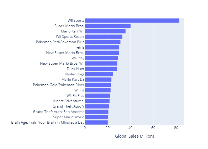

Top100 타이블 개발사 비율 pie chart (plotly)

global_top100_pub_pie = plex.pie(data_frame=top100_global,hole=0.3,
                             values='Global_Sales',names='Publisher')
global_top100_pub_pie.update_traces(textposition='inside', textinfo='percent+label')
global_top100_pub_pie.update_layout(annotations=[dict(text='Global',showarrow=False)])
global_top100_pub_pie.show()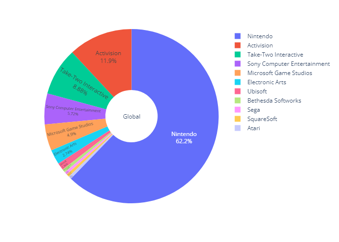

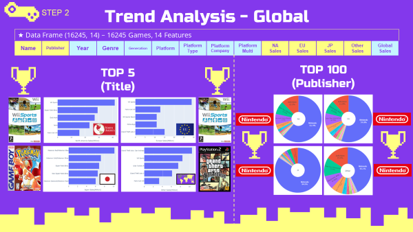
지역별 최고 매출 게임 및 개발사 분석

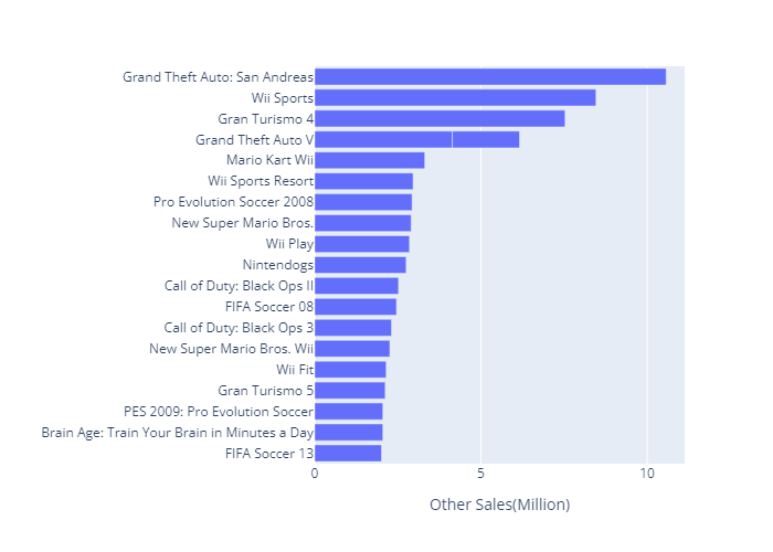
대륙별로 분석해도 닌텐도에서 개발한 게임들이 가장 높은 비율을 차지하였음.
그래프 소스 코드는 모든 지역이 같은 코드로 구성되어 있으므로, 본 블로그에서는 Other Country 소스 코드만 기록하겠음.
Other Country bar chart (plotly)

#데이터
top20_Ot = vgames.sort_values(by='Other_Sales',ascending=False).head(20).reset_index(drop=True)
top100_Ot = vgames.sort_values(by='Other_Sales',ascending=False).head(100).reset_index(drop=True)
#bar chart
Ot_top20_name = plex.bar(x=top20_Ot.Other_Sales,y=top20_Ot.Name)
Ot_top20_name.update_layout(yaxis=dict(autorange='reversed')
                       ,xaxis_title=dict(text='Other Sales(Million)')
                       ,yaxis_title=dict(text=''))
Ot_top20_name.show()

plotly graph는 조작가능한 interactive graph이기 때문에, ppt에는 Top20 plot을 드래그하여 잘라낸 Top5 그래프를 캡쳐하여 이용하였음.

Other Country pie chart (plotly)

#pie chart
Ot_top100_pub_pie = plex.pie(data_frame=top100_Ot,hole=0.3,
                             values='Global_Sales',names='Publisher')
Ot_top100_pub_pie.update_traces(textposition='inside', textinfo='percent+label')
Ot_top100_pub_pie.update_layout(annotations=[dict(text='Other',showarrow=False)])
Ot_top100_pub_pie.show()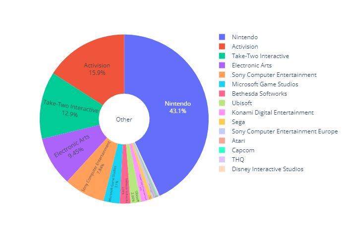

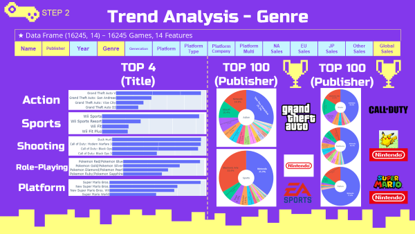
3-2. Genre Trend 장르 트렌드 분석

Global 장르 트렌드

전세계적으로 액션, 스포츠, 슈팅, 롤플레잉, 플랫폼 장르 순으로 선호도가 높게 나타남.
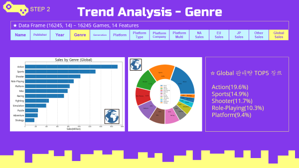
장르 Grouping

df_Genre = vgames.groupby(['Genre'],as_index=False)[Sales_list].sum()

bar chart (matplotlib)

#global barplot
Genre_sort = df_Genre.sort_values(by='Global_Sales',ascending=True).reset_index(drop=True)
plot_index = np.arange(len(Genre_sort.Genre))
plt.figure(figsize=(12,8))
plt.barh(plot_index,Genre_sort.Global_Sales)
plt.title('Sales by Genre (Global)',fontsize=24)
plt.xlabel('Sales(Million)',fontsize=16)
plt.ylabel('')
plt.yticks(plot_index,Genre_sort.Genre,fontsize=16)
plt.grid(True,axis='x',linestyle='--')
plt.xlim([0,1800])
plt.show()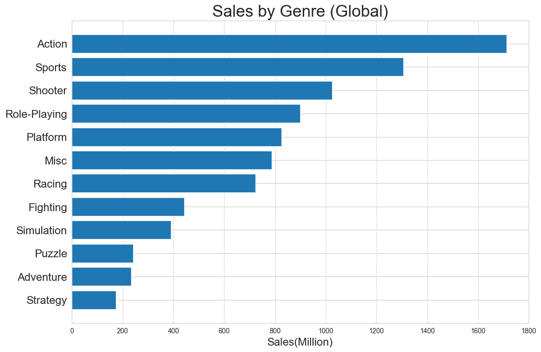

pie chart (matplotlib)

#Global pie chart
explode = np.repeat(0.025,12)
wedgeprops = {'width': 0.5, 'edgecolor': 'w', 'linewidth': 1.5}
textprops={'size':12}
Genre_sort2 = df_Genre.sort_values(by='Global_Sales',ascending=False).reset_index(drop=True)
plt.figure(figsize=(12,12))
plt.pie(Genre_sort2.Global_Sales,
		labels=Genre_sort2.Genre,
        labeldistance=0.725,
        startangle=0,
        autopct='%.1f%%',
        explode=explode,
        wedgeprops=wedgeprops,
        textprops=textprops)
plt.legend(loc='center')
plt.show()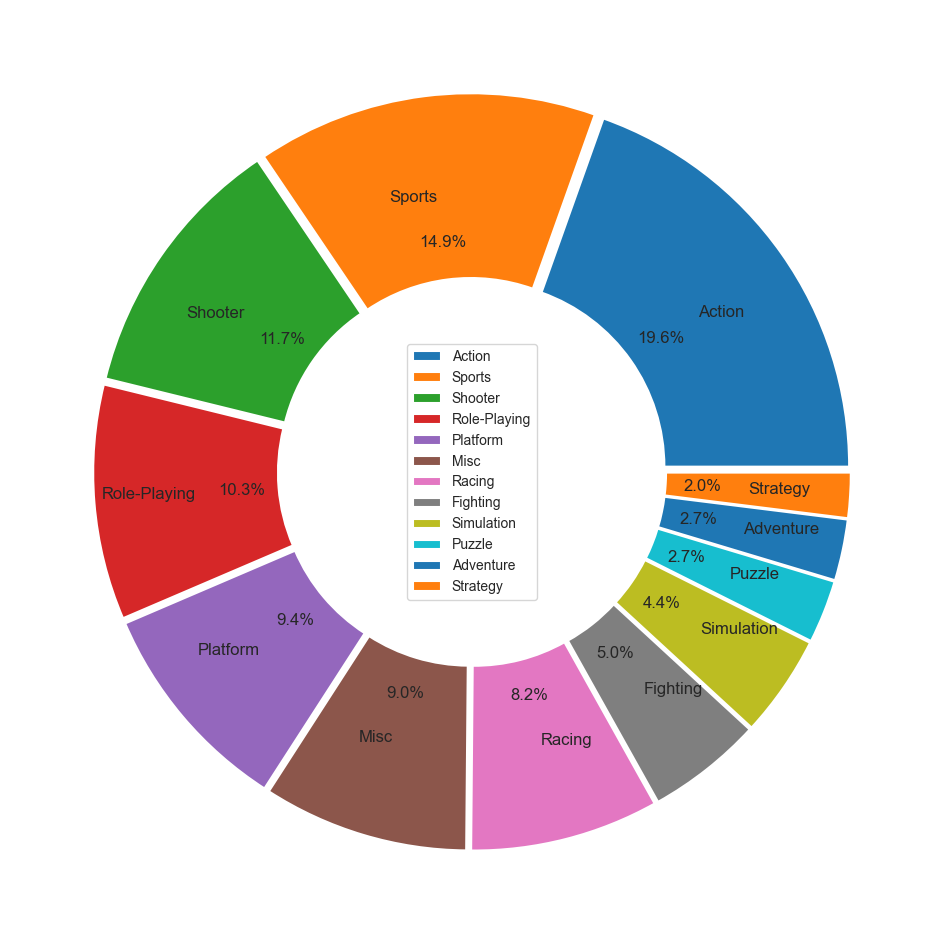

지역별 장르 선호도

일본에서는 롤플레잉 장르가 가장 선호도가 높았고, 슈팅장르가 가장 낮은 선호도를 보임.
그외 모든 지역에서는 액션, 스포츠, 슈팅 장르 순으로 선호도가 높게 나타남.
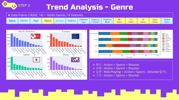
지역별 장르 선호도 stack bar plot (matplotlib)

#지역별 장르 데이터
Genre_sort2 = df_Genre.sort_values(by='Global_Sales',ascending=False).reset_index(drop=True)
genre_stack = Genre_sort2.iloc[:,:-1].T.iloc[1:,:]
genre_stack.columns = Genre_sort2.Genre
genre_per = genre_stack.div(genre_stack.sum(axis=1),axis=0)*100
#지역별 stack barplot
genre_per_ud = genre_per.loc[::-1]
genre_per_ud.index = ['Other','Japan','Europe','North America']
genre_per_ud.plot(kind = 'barh',stacked='True',figsize=(10,4))
plt.grid(True,axis='x',linestyle='--')
plt.xlabel('Percent(%)')
plt.legend(loc=(1.02,0.1))
plt.show();

지역별 장르 선호도 bar chart (plotly)

#지역별 장르 데이터
Genre_NA = df_Genre.sort_values(by='NA_Sales',ascending=False).reset_index(drop=True)
Genre_EU = df_Genre.sort_values(by='EU_Sales',ascending=False).reset_index(drop=True)
Genre_JP = df_Genre.sort_values(by='JP_Sales',ascending=False).reset_index(drop=True)
Genre_Ot = df_Genre.sort_values(by='Other_Sales',ascending=False).reset_index(drop=True)
#지역별 barplot
region_genre = plsub(rows=2,cols=2,subplot_titles=('North America','Europe','Japan','Other'))
region_genre.add_bar(x= Genre_NA.Genre,y=Genre_NA.NA_Sales,name='North America',row=1,col=1)
region_genre.add_bar(x= Genre_EU.Genre,y=Genre_EU.EU_Sales,name='Europe',row=1,col=2)
region_genre.add_bar(x= Genre_JP.Genre,y=Genre_JP.JP_Sales,name='Japan',row=2,col=1)
region_genre.add_bar(x= Genre_Ot.Genre,y=Genre_Ot.Other_Sales,name='Other',row=2,col=2)
region_genre.update_xaxes(tickangle= 45)
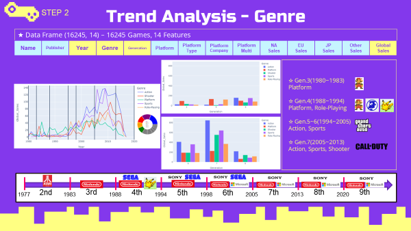
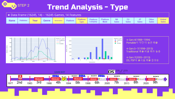
region_genre.show()

연도별 장르 선호도 (top5 장르)

3세대에서는 플랫폼 장르가 높은 선호도를 보임
- 3세대 플랫폼 장르 대표작
  - 닌텐도 NES(패미컴) 마리오 브라더스
4세대에서는 플랫폼 장르와 롤플레잉 장르가 높은 매출을 보임
- 4세대 플랫폼 장르 대표작
  - 닌텐도 SNES(슈퍼패미컴) 슈퍼 마리오 월드
  - 세가 GENESIS(메가드라이드) 소닉 더 헤지혹
- 4세대 롤플레잉 장르 대표작
  - 닌텐도 GAMEBOY(게임보이) 포켓몬스터 (레드,블루,그린)
5~6세대에서는 액션 장르와 스포츠 장르가 높은 선호도를 보임
- 액션장르 대표작
  - Take-Two Interactive사의 GTA(Grand-Theft-Auto) 시리즈
7세대에서 슈팅 장르의 선호도가 급증함
- 슈팅장르 대표작
  - Activision사의 Call of Duty 시리즈

연도(세대)별 Genre(TOP5) 데이터

top5genre = ['Action','Sports','Shooter','Role-Playing','Platform']
df_top5_genre_year = df_genre_year[df_genre_year.Genre.isin(top5genre)]
df_top5_genre_gen = df_genre_gen[df_genre_gen.Genre.isin(top5genre)]

연도별 Genre(TOP5) 선호도 line chart (plotly)

top5_year_genre = plex.line(data_frame=df_top5_genre_year,
							x='Year',
                            y='Global_Sales',
                            color='Genre',
                            title='Top5 Genre Sales Trend(Global)')
top5_year_genre.add_vline(1980)
top5_year_genre.add_vline(1983)
top5_year_genre.add_vline(1988)
top5_year_genre.add_vline(1995)
top5_year_genre.add_vline(1998)
top5_year_genre.add_vline(2005)
top5_year_genre.add_vline(2013)
top5_year_genre.add_vline(2020)
top5_year_genre.show()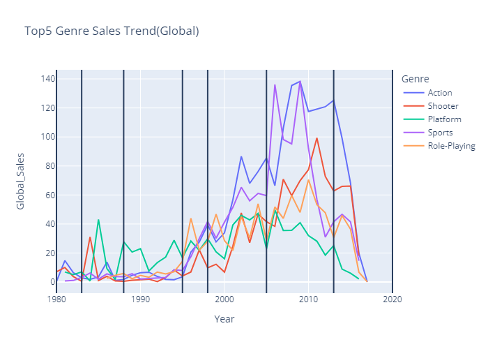

세대별 Genre(TOP5) 선호도 bar chart (plotly)

top5_gen_genre = plex.bar(data_frame=df_top5_genre_gen,
                          x='Generation',
                          y='Global_Sales',
                          color='Genre',
                          title='Top5 Genre Sales Trend(Global)',
                          barmode='group')
top5_gen_genre.show()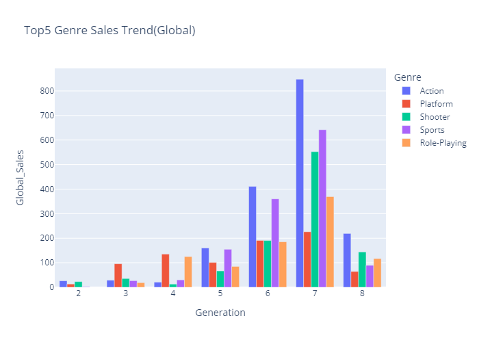

장르별 최고매출 게임, 개발사 분석 (top5 장르)

소드코드는 Global Sales Trend 최고매출 분석 소스코드와 같은 방식으로 진행하였으므로 ppt로 대체하겠음.
위에서 언급한 게임과 개발사들이 각 장르별로 높은 매출을 기록하였음.

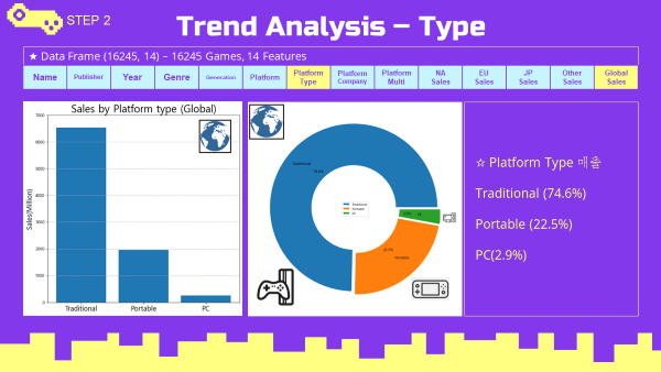
3-3. Platform Type Trend 플랫폼 타입 트렌드 분석

Global 플랫폼 타입 트렌드

거치형(Traditional)타입의 플랫폼이 높은 매출 비율을 차지함.

플랫폼 타입 데이터 Grouping

df_type = vgames.groupby(['Platform_type'],as_index=False)[Sales_list].sum()
df_type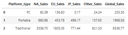

플랫폼 타입 매출 bar chart (matplotlib)

#global barplot
type_sort = df_type.sort_values(by='Global_Sales',ascending=False).reset_index(drop=True)
type_index = np.arange(len(type_sort.Platform_type))
plt.figure(figsize=(8,8))
plt.bar(type_index,type_sort.Global_Sales)
plt.title('Sales by Platform type (Global)',fontsize=24)
plt.xlabel('')
plt.ylabel('Sales(Million)',fontsize=16)
plt.xticks(type_index,type_sort.Platform_type,fontsize=16)
plt.grid(True,axis='y',linestyle='--')
plt.ylim([0,7000])
plt.show()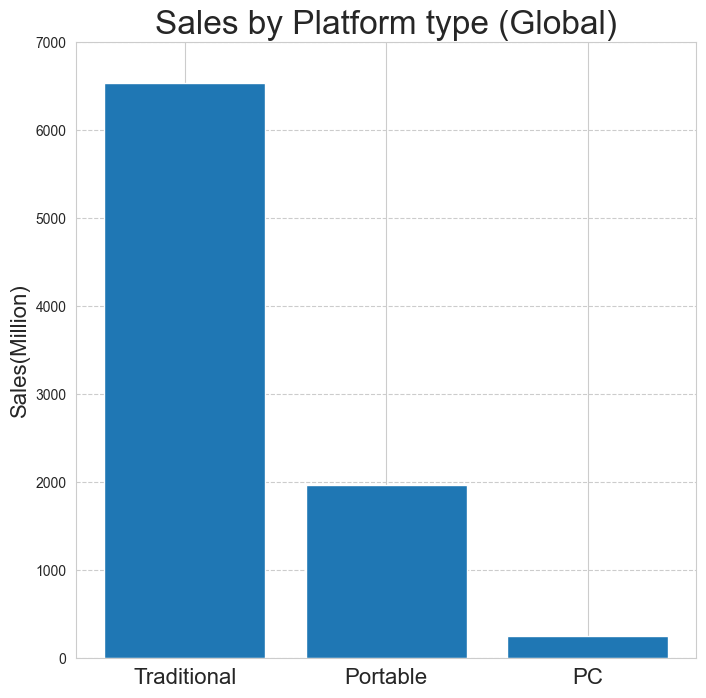

플랫폼 타입 매출 pie chart (matplotlib)

#Global pie chart
explode = np.repeat(0.025,3)
wedgeprops = {'width': 0.5, 'edgecolor': 'w', 'linewidth': 1.5}
textprops={'size':12}
type_sort2 = df_type.sort_values(by='Global_Sales',ascending=False).reset_index(drop=True)
plt.figure(figsize=(12,12))
plt.pie(type_sort2.Global_Sales,
		labels=type_sort2.Platform_type,
        labeldistance=0.725,startangle=0,
        autopct='%.1f%%',
        explode=explode,
        wedgeprops=wedgeprops,
        textprops=textprops)
plt.legend(loc='center')
plt.show()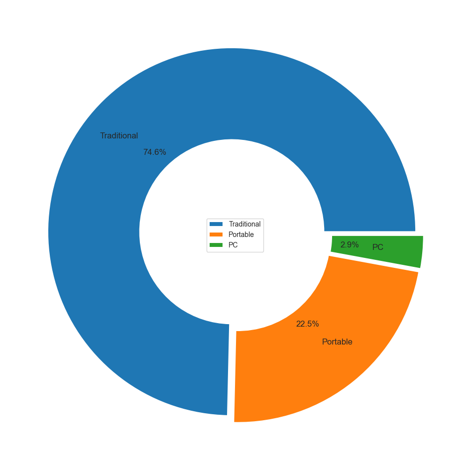

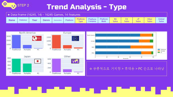
지역별 플랫폼 타입 트렌드

지역에 관계없이 거치형, 휴대용, PC 순으로 매출이 높게 나타났음.

지역별 플랫폼 타입 stack barplot (matplotlib)

#데이터
type_stack = type_sort2.iloc[:,:-1].T.iloc[1:,:]
type_stack.columns = type_sort2.Platform_type
type_per = type_stack.div(type_stack.sum(axis=1),axis=0)*100
#지역별 stack barplot
type_per_ud = type_per.loc[::-1]
type_per_ud.index = ['Other','Japan','Europe','North America']
type_per_ud.plot(kind = 'barh',stacked='True',figsize=(10,4))
plt.grid(True,axis='x',linestyle='--')
plt.xlabel('Percent(%)')
plt.legend(loc=(1.02,0.1))
plt.show();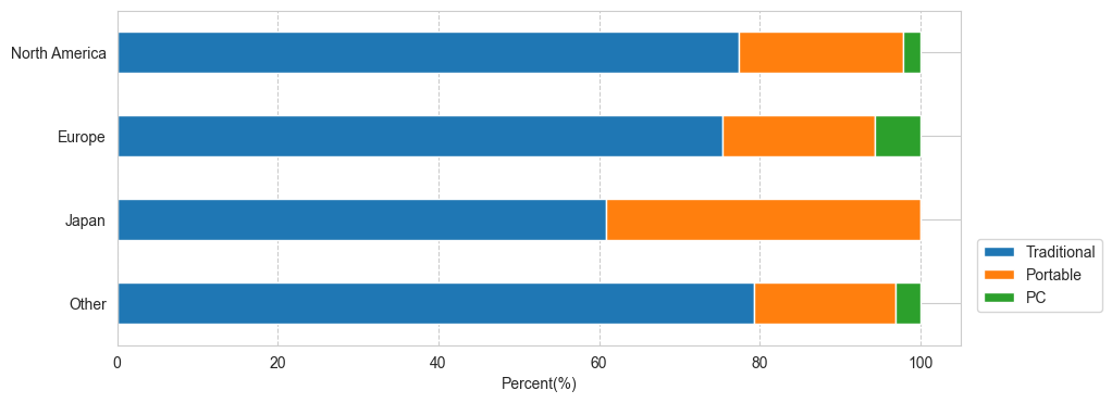

지역별 플랫폼 타입 bar plot (plotly)

#지역별 barplot 데이터
type_NA = df_type.sort_values(by='NA_Sales',ascending=False).reset_index(drop=True)
type_EU = df_type.sort_values(by='EU_Sales',ascending=False).reset_index(drop=True)
type_JP = df_type.sort_values(by='JP_Sales',ascending=False).reset_index(drop=True)
type_Ot = df_type.sort_values(by='Other_Sales',ascending=False).reset_index(drop=True)
#지역별 barplot
region_type = plsub(rows=2,cols=2,subplot_titles=('North America','Europe','Japan','Other'))
region_type.add_bar(x= type_NA.Platform_type,y=type_NA.NA_Sales,name='North America',row=1,col=1)
region_type.add_bar(x= type_EU.Platform_type,y=type_EU.EU_Sales,name='Europe',row=1,col=2)
region_type.add_bar(x= type_JP.Platform_type,y=type_JP.JP_Sales,name='Japan',row=2,col=1)
region_type.add_bar(x= type_Ot.Platform_type,y=type_Ot.Other_Sales,name='Other',row=2,col=2)
region_type.update_xaxes(tickangle= 0)
region_type.show()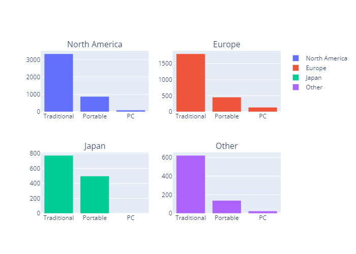

연도(세대)별 플랫폼 타입 트렌드

전반적으로 거치형 게임기의 매출이 높은 비율을 차지함

연도(세대)별 플랫폼 타입 데이터

df_type_year = vgames.groupby(['Year','Platform_type'],as_index=False).sum()
df_type_gen = vgames.groupby(['Generation','Platform_type'],as_index=False).sum()

연도별 플랫폼 타입 line chart (plotly)

year_type = plex.line(data_frame=df_type_year,
						x='Year',
                        y='Global_Sales',
                        color='Platform_type',
                        title='Platform type Sales Trend(Global)')
year_type.add_vline(1980)
year_type.add_vline(1983)
year_type.add_vline(1988)
year_type.add_vline(1994)
year_type.add_vline(1998)
year_type.add_vline(2005)
year_type.add_vline(2013)
year_type.add_vline(2020)
year_type.show()

세대별 플랫폼 타입 bar chart (plotly)

gen_type = plex.bar(data_frame=df_type_gen,
                    x='Generation',
                    y='Global_Sales',
                    color='Platform_type',
                    title='Platform type Sales Trend(Global)',
                    barmode='group')
gen_type.show()

플랫폼 타입별 최고매출 게임, 개발사 분석

소드코드는 Global Sales Trend 최고매출 분석 소스코드와 같은 방식으로 진행하였으므로 ppt로 대체하겠음.
거치형과 휴대용 게임 모두 닌텐도의 매출 비율이 높게 나타남.
PC게임에서는 EA와 Activision(Blizzard)의 매출 비율이 높게 나타남.

3-4. Platform Company Trend 플랫폼 기업 트렌드 분석

Global 플랫폼 기업 트렌드

닌텐도와 소니의 양강구도에서 마이크로소프트가 추격하는 형태

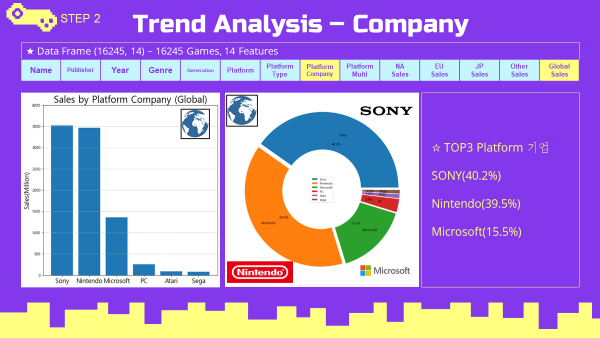
Global 플랫폼 기업 데이터

df_company = vgames.groupby(['Platform_company'],as_index=False)[Sales_list].sum()
df_company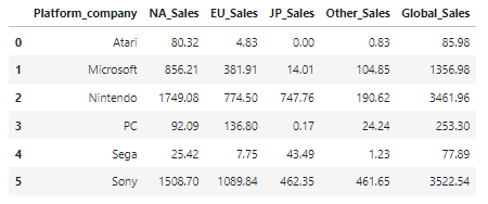

Global 플랫폼 기업 bar chart (matplotlib)

#global barplot
company_sort = df_company.sort_values(by='Global_Sales',ascending=False).reset_index(drop=True)
company_index = np.arange(len(company_sort.Platform_company))
plt.figure(figsize=(8,8))
plt.bar(company_index,company_sort.Global_Sales)
plt.title('Sales by Platform Company (Global)',fontsize=24)
plt.xlabel('')
plt.ylabel('Sales(Million)',fontsize=16)
plt.xticks(company_index,company_sort.Platform_company,fontsize=16)
plt.grid(True, axis='y',linestyle='--')
plt.ylim([0,4000])
plt.show()

Global 플랫폼 기업 pie chart (matplotlib)

#Global pie chart
explode = np.repeat(0.025,6)
wedgeprops = {'width': 0.5, 'edgecolor': 'w', 'linewidth': 1.5}
textprops={'size':12}
company_sort2 = df_company.sort_values(by='Global_Sales',ascending=False).reset_index(drop=True)
plt.figure(figsize=(12,12))
plt.pie(company_sort2.Global_Sales,
		labels=company_sort2.Platform_company,
        labeldistance=0.725,
        startangle=0,
        autopct='%.1f%%',
        explode=explode,
        wedgeprops=wedgeprops,
        textprops=textprops)
plt.legend(loc='center')
plt.show()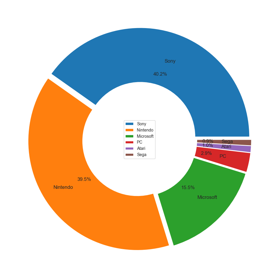

지역별 플랫폼 기업 트렌드

북미와 일본에서는 닌텐도가 가장 높은 매출
유럽과 그외지역에서는 소니가 가장 높은 매출

지역별 플랫폼 기업 stack bar chart (matplotlib)

#지역별 stack barplot
company_stack = company_sort2.iloc[:,:-1].T.iloc[1:,:]
company_stack.columns = company_sort2.Platform_company
company_per = company_stack.div(company_stack.sum(axis=1),axis=0)*100
company_per_ud = company_per.loc[::-1]
company_per_ud.index = ['Other','Japan','Europe','North America']
company_per_ud.plot(kind = 'barh',stacked='True',figsize=(10,4))
plt.grid(True,axis='x',linestyle='--')
plt.xlabel('Percent(%)')
plt.legend(loc=(1.02,0.1))
plt.show();

지역별 플랫폼 기업 bar chart (plotly)

#지역별 barplot 데이터
company_NA = df_company.sort_values(by='NA_Sales',ascending=False).reset_index(drop=True)
company_EU = df_company.sort_values(by='EU_Sales',ascending=False).reset_index(drop=True)
company_JP = df_company.sort_values(by='JP_Sales',ascending=False).reset_index(drop=True)
company_Ot = df_company.sort_values(by='Other_Sales',ascending=False).reset_index(drop=True)
#지역별 barplot
region_company = plsub(rows=2,cols=2,subplot_titles=('North America','Europe','Japan','Other'))
region_company.add_bar(x= company_NA.Platform_company,y=company_NA.NA_Sales,name='North America',row=1,col=1)
region_company.add_bar(x= company_EU.Platform_company,y=company_EU.EU_Sales,name='Europe',row=1,col=2)
region_company.add_bar(x= company_JP.Platform_company,y=company_JP.JP_Sales,name='Japan',row=2,col=1)
region_company.add_bar(x= company_Ot.Platform_company,y=company_Ot.Other_Sales,name='Other',row=2,col=2)
region_company.update_xaxes(tickangle= 0)
region_company.show()

연도(세대)별 플랫폼 기업 트렌드

Gen.2 (1977~1983)
- Atari 의 독점
Gen.3 (1983~1988)
- Atari 의 몰락, Nintendo의 독점
Gen.4 (1988~1994)
- PC게임 등장, Sega출전 But Nintendo의 압승
Gen.5 (1994~1998)
- SONY의 등장과 함께 SONY의 압도적 승리
Gen.6 (1998~2005)
- Microsoft의 참전 but SONY의 여전한 압승
Gen.7 (2005~2013)
- DS, Wii의 성공으로 Nintendo의 높은 매출비율
- 콘솔시장의 전성기, N S M 삼국지시대
Gen.8 (2013~2020)
- 스마트폰 게임시장 성장에 따라 콘솔시장 축소

연도(세대)별 플랫폼 기업 Grouping

df_company_year = vgames.groupby(['Year','Platform_company'],as_index=False).sum()
df_company_gen = vgames.groupby(['Generation','Platform_company'],as_index=False).sum()

연도별 플랫폼 기업 매출 line chart (plotly)

year_company = plex.line(data_frame=df_company_year,
						x='Year',
                        y='Global_Sales',
                        color='Platform_company',
                        title='Platform company Sales Trend(Global)')
year_company.add_vline(1980)
year_company.add_vline(1983)
year_company.add_vline(1988)
year_company.add_vline(1994)
year_company.add_vline(1998)
year_company.add_vline(2005)
year_company.add_vline(2013)
year_company.add_vline(2020)
year_company.show()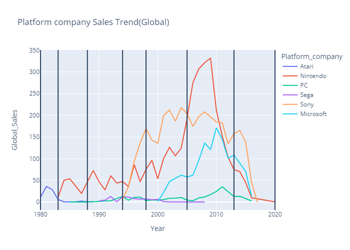

장르별 플랫폼 기업 매출 line chart (plotly)

gen_company = plex.bar(data_frame=df_company_gen,
                       x='Generation',
                       y='Global_Sales',
                       color='Platform_company',
                       title='Platform company Sales Trend(Global)',
                       barmode='group')
gen_company.show()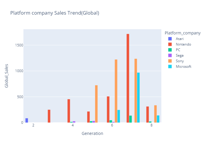

플랫폼 기업별 최고매출 게임, 개발사 분석

소드코드는 Global Sales Trend 최고매출 분석 소스코드와 같은 방식으로 진행하였으므로 ppt로 대체하겠음.
닌텐도 플랫폼 게임은 닌텐도에서 직접 개발한 게임들이 압도적으로 높은 매출을 차지함.
소니와 마이크로소프트 플랫폼은 개방형 플랫폼이다보니, 플랫폼 기업에서 개발한 게임외에 EA, Take-Two, Activision 사의 게임들도 비슷한 비율로 높은 매출을 차지함

3-5. 트렌드 분석 요약 정리

모든 지역에서 매출이 2010년 이후에 하락세를 보임 (스마트폰 출시의 영향으로 보임)
장르 선호도는 액션, 스포츠, 슈팅 순이지만, 일본에서는 롤플레잉 장르가 가장 높은 선호도를 보임
전반적으로 거치형 게임기의 매출이 높음
플랫폼은 현재 소니와 닌텐도의 양강구도에서 마이크로소프트가 추격하는 형태

04. Hypothesis Test 가설 검정

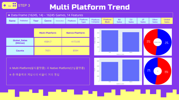
4-0. 멀티플랫폼 트렌드

멀티플랫폼 총매출, 타이틀 수 비교

단일플랫폼과 멀티플랫폼의 총 매출비율과 게임 수가 거의 비슷하게 나타남.

멀티플랫폼 트렌드 데이터

vgames_sum = vgames.groupby('Platform_Multi',as_index=False)[Sales_list].sum()
display(vgames_sum)
vgames_count = vgames.groupby('Platform_Multi',as_index=False)[Sales_list].count()
display(vgames_count)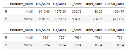

총매출 비교 bar chart (plotly)

multi_global_sum = plex.bar(data_frame=vgames_sum,x='Platform_Multi',y='Global_Sales')
multi_global_sum.show()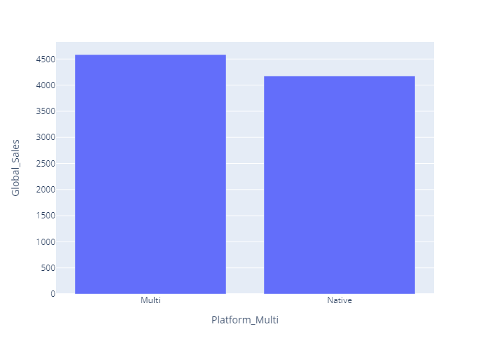

총매출 비교 pie chart (plotly)

multi_global_sum_pie = plex.pie(data_frame=vgames_sum,hole=0.3,
                             values='Global_Sales',
                             names='Platform_Multi', 
                             color='Platform_Multi',
                             color_discrete_map={'Native':'red','Multi':'blue'})
multi_global_sum_pie.update_traces(textposition='inside', textinfo='percent+label')
multi_global_sum_pie.update_layout(annotations=[dict(text='Global_Sales',showarrow=False)])
multi_global_sum_pie.show()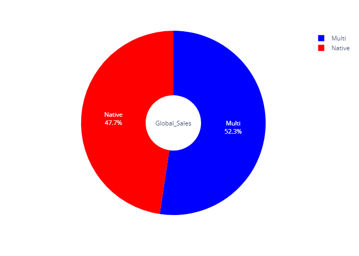

타이틀 수 비교 bar chart (plotly)

multi_global_n = plex.bar(data_frame=vgames_count,x='Platform_Multi',y='Global_Sales')
multi_global_n.update_layout(yaxis_title=dict(text='Count'))
multi_global_n.show()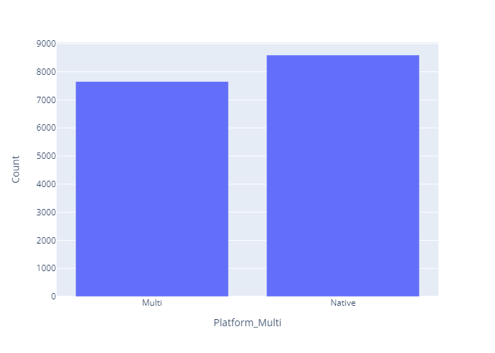

타이틀 수 비교 pie chart (plotly)

multi_global_n_pie = plex.pie(data_frame=vgames_count,hole=0.3,
                             values='Global_Sales',names='Platform_Multi', color='Platform_Multi',
                             color_discrete_map={'Native':'red','Multi':'blue'})
multi_global_n_pie.update_traces(textposition='inside', textinfo='percent+label')
multi_global_n_pie.update_layout(annotations=[dict(text='N',showarrow=False)])
multi_global_n_pie.show()

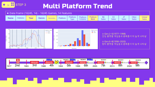
멀티플랫폼 연도(세대)별 트렌드

2~5세대(1977~1998) - 단일플랫폼의 총매출이 더 높음
6~8세대(1988~2020) - 멀티플랫폼의 총매출이 더 높음

연도(세대)별 Grouping

df_multi_year = vgames.groupby(['Year','Platform_Multi'],as_index=False)[Sales_list].sum()
df_multi_gen = vgames.groupby(['Generation','Platform_Multi'],as_index=False)[Sales_list].sum()

연도별 멀티플랫폼 트렌드 line chart (plotly)

year_multi = plex.line(data_frame=df_multi_year,
						x='Year',y='Global_Sales',
                       color='Platform_Multi',
                       title='Multi Platform Sales Trend(Global)')
year_multi.add_vline(1980)
year_multi.add_vline(1983)
year_multi.add_vline(1988)
year_multi.add_vline(1994)
year_multi.add_vline(1998)
year_multi.add_vline(2005)
year_multi.add_vline(2013)
year_multi.add_vline(2020)
year_multi.show()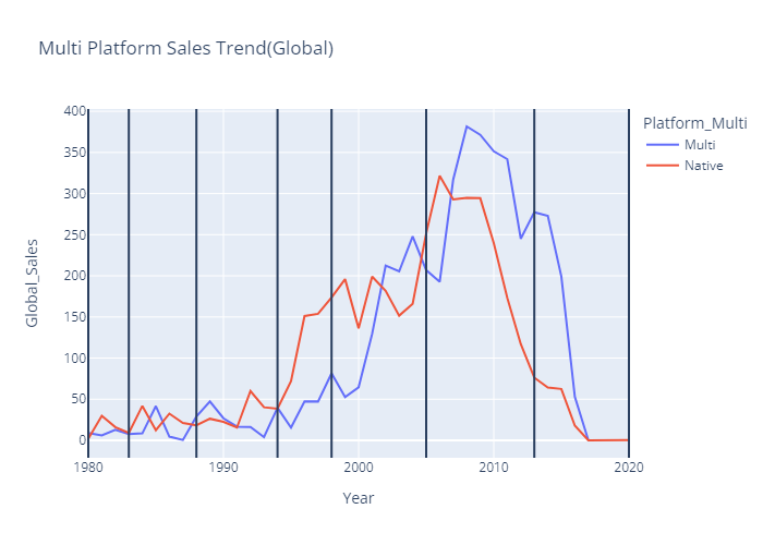

세대별 멀티플랫폼 트렌드 bar chart (plotly)

gen_multi = plex.bar(data_frame=df_multi_gen,
                       x='Generation',y='Global_Sales',
                       color='Platform_Multi',
                       title='Multi Platform Sales Trend(Global)',
                       barmode='group')
gen_multi.show()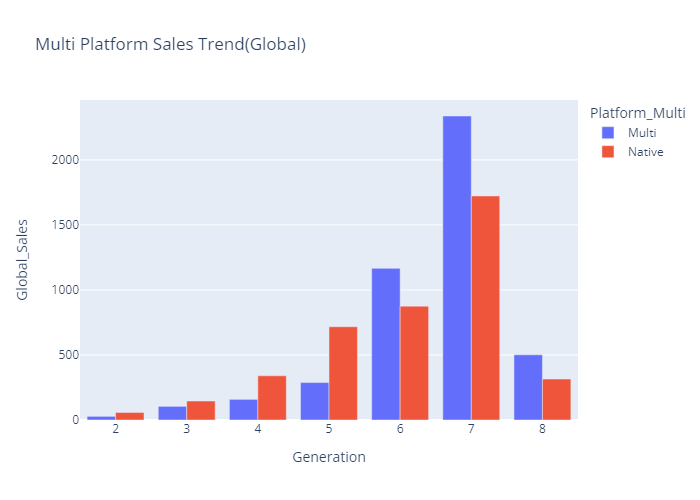

멀티플랫폼 최고매출 트렌드

소드코드는 Global Sales Trend 최고매출 분석 소스코드와 같은 방식으로 진행하였으므로 ppt로 대체하겠음.
단일플랫폼은 플랫폼 기업들이 직접 개발한 게임들이 높은 매출 비율을 차지함.
멀티플랫폼은 Activision, EA, 닌텐도, Take-Two 순으로 높은 매출 비율을 차지함.

4-1. 멀티플랫폼 가설검정

Global 멀티플랫폼 가설검정

귀무가설(H0) : 멀티플랫폼 평균매출이 단일플랫폼 평균매출보다 크지 않다.
대립가설(Ha) : 멀티플랫폼 평균매출이 단일플랫폼 평균매출보다 크다.
Levene 등분산 검정결과 : p-value = 0.006, 두 집단의 분산이 같지 않음.
One-tailed T-test (equal_var=False) 결과
- 멀티 플랫폼 평균매출이 단일플랫폼 평균매출보다 유의미하게 크다.

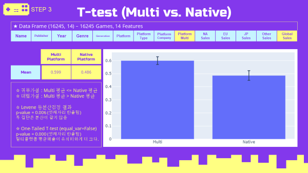
평균 데이터

vgames_mean = vgames.groupby('Platform_Multi',as_index=False)[Sales_list].mean()
display(vgames_mean)

평균 매출 bar chart (plotly)

# error bar
def mean_conf_inter(data, confidence=0.95):
    data = np.array(data)
    m = np.mean(data)
    n = len(data)
    s = stats.sem(data)
    i = stats.t.ppf((1+confidence)/2,n-1)*s
    return i
vgames_native = vgames.query('Platform_Multi == "Native"')
vgames_multi = vgames.query('Platform_Multi == "Multi"')
error_bar_native = mean_conf_inter(vgames_native.Global_Sales)
error_bar_multi = mean_conf_inter(vgames_multi.Global_Sales)
print(error_bar_native)
print(error_bar_multi)
# error bar output
'''
0.03694679704961938
0.02969598890309412
'''
#bar chart with error bar
multi_global_mean_error = go.Figure(data=[go.Bar(x=vgames_mean.Platform_Multi, y=vgames_mean.Global_Sales,
                                                error_y=dict(type='data', array=[error_bar_multi,error_bar_native])
                                                )])
multi_global_mean_error.show()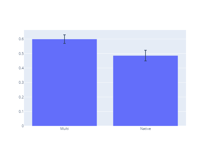

등분산 검정 & One-Tailed T-test (scipy.stats)

vgames_native = vgames.query('Platform_Multi == "Native"')
vgames_multi = vgames.query('Platform_Multi == "Multi"')
se_native_global = vgames_native.Global_Sales
se_multi_global = vgames_multi.Global_Sales
levene_multi = stats.levene(se_native_global,se_multi_global).pvalue
print('levene 등분산검정 p-value : {:.3f}'.format(levene_multi))
ttest_multi = stats.ttest_ind(se_multi_global,se_native_global,alternative='greater',equal_var=False).pvalue
print('T-test 단측검정 p-value : {:.3f}'.format(ttest_multi))
#output
'''
levene 등분산검정 p-value : 0.006
T-test 단측검정 p-value : 0.000
'''

지역별 멀티플랫폼 가설검정

일본에서는 단일 플랫폼 게임의 평균 매출이 유의미하게 더 높았음.
그외 모든 지역에서는 멀티 플랫폼 게임의 평균 매출이 유의미하게 더 높았음.
지역별 T-test 소스코드는 Global 가설검정과 동일한 방식으로 진행하였으므로, 본 블로그에서는 ppt로 대체함.

지역별 멀티플랫폼 bar chart (plotly)

#지역별 barplot 데이터
multi_NA = vgames_mean.sort_values(by='NA_Sales',ascending=False).reset_index(drop=True)
multi_EU = vgames_mean.sort_values(by='EU_Sales',ascending=False).reset_index(drop=True)
multi_JP = vgames_mean.sort_values(by='JP_Sales',ascending=False).reset_index(drop=True)
multi_Ot = vgames_mean.sort_values(by='Other_Sales',ascending=False).reset_index(drop=True)
#지역별 barplot
region_multi = plsub(rows=2,cols=2,subplot_titles=('North America','Europe','Japan','Other'))
region_multi.add_bar(x= multi_NA.Platform_Multi,y=multi_NA.NA_Sales,name='North America',row=1,col=1)
region_multi.add_bar(x= multi_EU.Platform_Multi,y=multi_EU.EU_Sales,name='Europe',row=1,col=2)
region_multi.add_bar(x= multi_JP.Platform_Multi,y=multi_JP.JP_Sales,name='Japan',row=2,col=1)
region_multi.add_bar(x= multi_Ot.Platform_Multi,y=multi_Ot.Other_Sales,name='Other',row=2,col=2)
region_multi.update_xaxes(tickangle= 0)
region_multi.show()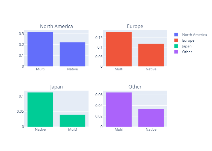

4-2. 멀티플랫폼 가설검정 요약정리

세계적으로는 멀티플랫폼의 평균매출이 유의미하게 더 높았음.
지역별로는 일본에서만 반대로 단일플랫폼의 평균매출이 유의미하게 더 높게 나타났음.

05. Conclusion 결론

5-1. Summary 최종 요약

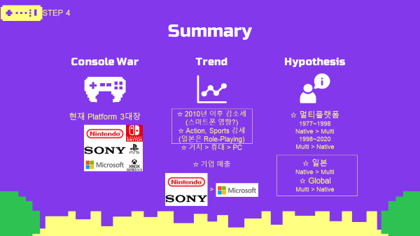
현재 플랫폼 게임 시장은 닌텐도, 소니, 마이크로소프트가 이끌어 가고있음.
2010년 이후에 매출량의 감소세를 보이는데, 개인적으로 스마트폰 게임 시장의 성장과 연관이 크다 알려져 있음.
장르는 액션장르와 스포츠장르가 선호도가 높고, 일본에서는 롤플레잉 장르가 선호도가 높음.
멀티플랫폼에 대한 가설검정 결과, 일본을 제외하고 전세계적으로는 멀티플랫폼이 평균매출이 유의미하게 높았음.

5-2. Conclusion 결론 및 인사이트 도출

장르는 일본 시장까지 고려하면, 액션장르와 스포츠장르가 무난할 것으로 보임.
플랫폼 형태는 현재 전체적으로 매출이 하락세이므로, 스마트폰 모바일 게임 시장에 대한 추가적인 조사가 필요해 보임.
플랫폼 기업은 아직 닌텐도와 소니의 양강구도가 유지 중이지만, 지속적인 트렌드 조사가 필요함.
멀티플랫폼 개발에 있어서 세계적으로는 멀티플랫폼이 더 높은 매출을 기대해볼 수 있음.
- 일본 시장을 노릴 경우엔 단일 플랫폼으로 출시하는 것이 유리할 것으로 보임.

5-3. Retrospective 회고

본 프로젝트를 마치고 그동안 이후 Section을 진행하느라 바빠서 이제서야 이 프로젝트를 정리해보게 되었음..
코드스테이츠에서 정한 발표 영상 시간이 8분 밖에 되지 않아서, 발표 영상에서는 많은 부분 스킵했었지만, 블로그를 통해 전하고자했던 내용을 모두 담아 낼 수 있어서 좋았음.
비록 정해진 주제와 정해진 데이터셋을 이용한 프로젝트였지만, 어린시절부터 닌텐도 게임을 쭉 즐겨왔던 입장에서는 도메인 지식을 활용하기 좋은 주제여서 개인적으로는 즐겁게 프로젝트를 수행할 수 있었음.
프로젝트 내용을 정리해보면서 복습도 많이 되었고, 프로젝트 진행할 땐 못봤던 오타나 오류도 다시 볼 수 있어서 좋았음.
코드를 쭉 정리하면서 지금이라면 조금 더 효율적으로 코드를 짜서 진행했을 수도 있겠구나 하는 생각이 많이 들었지만, 그래도 전반적으로는 만족스러웠던 코드였다 생각함.
코치에게 받은 피드백 중 지적받았던 점이 데이터셋에 대한 설명 부족, 발표자료의 양식에 쓰인 색 구성이었고, 이 부분은 본인도 공감하는 부분으로써 아쉬움이 남았었던 부분이라서 다음 프로젝트부터는 이러한 피드백을 최대한 반영하려고 노력하였음.
앞으로도 공부할 것과 복습해야할 것이 잔뜩 쌓여있지만, 이렇게라도 진행했던 프로젝트를 되돌아보는 시간을 가질 수 있어 좋았고, 앞으로도 쭉 공부를 열심히 해야겠다는 다짐을 다시 하게 될 수 있는 의미있는 시간이었음.
아자아자 파이팅!

Kyung Jae, Cheong

Machine Learning Engineer ( AI Engineer )

다음 포스트

[Project] Video Game 기획 프로젝트

개인프로젝트

어떤 게임을 설계해야할까?

00. 프로젝트 개요

상황 가정 & 필수 포함 요소

프로젝트 목차

01. Introduction 서론

1-1. Console War(1977~) 배경지식 - 콘솔전쟁

1-2. Purposes 프로젝트 목표

1-3. Process 프로젝트 진행 절차

02. Data 데이터

2-1. Data Preprocessing 데이터 전처리

STEP0. Data Import 데이터 불러오기

STEP1. 결측치 처리

STEP2. 오류 데이터 확인, 대체

STEP3. 중복치 확인, 제거

STEP4. 전처리 데이터 저장

2-2. Feature Engineering 특성 조합

STEP0. Data Import 데이터 불러오기

STEP1. Global Sales feature 생성

STEP2. Platform type feature 생성

STEP3. Platform company feature 생성

STEP4. Generation feature 생성

STEP5. 멀티플랫폼 feature 생성

STEP6. 최종 데이터 저장

03. Trends in Video Game 트렌드 분석

시각화 패키지(라이브러리)

3-0. Data Import 데이터 불러오기

3-1. Global Sales Trend 전세계 판매량 트렌드 분석

글로벌 총 판매량

연도(세대)별 총 판매량

최고 매출 게임 및 개발사 분석

지역별 최고 매출 게임 및 개발사 분석

3-2. Genre Trend 장르 트렌드 분석

Global 장르 트렌드

지역별 장르 선호도

연도별 장르 선호도 (top5 장르)

장르별 최고매출 게임, 개발사 분석 (top5 장르)

3-3. Platform Type Trend 플랫폼 타입 트렌드 분석

Global 플랫폼 타입 트렌드

지역별 플랫폼 타입 트렌드

연도(세대)별 플랫폼 타입 트렌드

플랫폼 타입별 최고매출 게임, 개발사 분석

3-4. Platform Company Trend 플랫폼 기업 트렌드 분석

Global 플랫폼 기업 트렌드

지역별 플랫폼 기업 트렌드

연도(세대)별 플랫폼 기업 트렌드

플랫폼 기업별 최고매출 게임, 개발사 분석

3-5. 트렌드 분석 요약 정리

04. Hypothesis Test 가설 검정

4-0. 멀티플랫폼 트렌드

멀티플랫폼 총매출, 타이틀 수 비교

멀티플랫폼 연도(세대)별 트렌드

멀티플랫폼 최고매출 트렌드

4-1. 멀티플랫폼 가설검정

Global 멀티플랫폼 가설검정

지역별 멀티플랫폼 가설검정

4-2. 멀티플랫폼 가설검정 요약정리

05. Conclusion 결론

5-1. Summary 최종 요약

5-2. Conclusion 결론 및 인사이트 도출

5-3. Retrospective 회고

[Project] 한국형 고혈압 예측 모델 개발 - (1) Intro & Data Preparation

0개의 댓글