[머신러닝] 의사결정나무, 서포트벡터머신

이현지·2024년 11월 30일

R/머신러닝/딥러닝

목록 보기

15/16

1. 라이브러리 임포트 및 설정

import pandas as pd
import numpy as np
import os
import tarfile
from six.moves import urllib
import matplotlib.pyplot as plt

항상 동일한 결과를 위한 random.seed 값 설정
np.random.seed(42)

주피터 노트북 안에 그림이 나오도록 설정
%matplotlib inline

2. 데이터 다운로드 함수 정의 및 실행

깃허브를 통한 데이터 다운

URL에서 데이터를 다운로드하고 압축을 해제하는 함수 정의 및 실행.

DOWNLOAD_ROOT = "https://raw.githubusercontent.com/ageron/handson-ml/master/"

HOUSING_PATH = os.path.join("input", "housing")

HOUSING_URL = DOWNLOAD_ROOT + "datasets/housing/housing.tgz"

def fetch_housing_data(housing_url=HOUSING_URL, housing_path=HOUSING_PATH):
if not os.path.isdir(housing_path):
os.makedirs(housing_path)
tgz_path = os.path.join(housing_path, "housing.tgz")
urllib.request.urlretrieve(housing_url, tgz_path)
housing_tgz = tarfile.open(tgz_path)
housing_tgz.extractall(path=housing_path)
housing_tgz.close()

fetch_housing_data()

3. 데이터 로드 및 미리보기

SV 파일을 판다스를 사용해 로드하고, 데이터의 마지막 5개 행을 확인함.

housing = pd.read_csv("./input/housing/housing.csv")
housing.tail()

데이터 첫 5행 확인
housing.head(5)

데이터프레임의 열 이름을 확인해 데이터를 탐색함.

housing.columns

Index(['longitude', 'latitude', 'housing_median_age', 'total_rooms',
       'total_bedrooms', 'population', 'households', 'median_income',
       'median_house_value', 'ocean_proximity'],
      dtype='object')

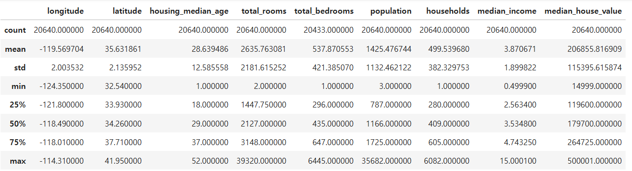
6. 데이터 통계 요약

데이터의 주요 통계 정보를 확인하여 평균, 표준편차, 최소/최대값 등 기본적인 통계를 분석함.

housing.describe()
#숫자형만 나옴

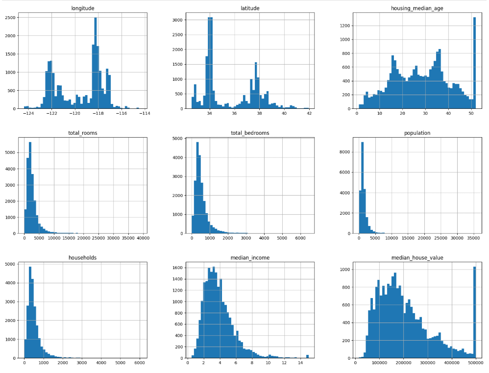
7. 데이터분포 확인

데이터를 히스토그램으로 시각화하여 각 특성의 분포를 분석함.

fig = housing.hist(bins=50, figsize=(20, 15))

plt.show()

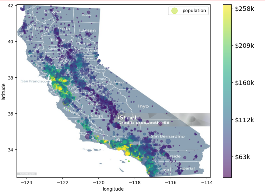
8. 위경도 기반 지리정보 시각화

주택 데이터를 지도에 시각화하여 인구 밀도와 중간 주택 가격의 공간적 분포를 확인함.

ax = housing.plot(
kind="scatter",
x="longitude",
y="latitude",
figsize=(10, 7),
s=housing["population"] / 100,
label="population",
c="median_house_value",
cmap=plt.get_cmap(),
colorbar=False,
alpha=0.5,
)

plt.imshow(california_img, extent=[-124.55, -113.80, 32.45, 42.05], alpha=0.6)

plt.show()

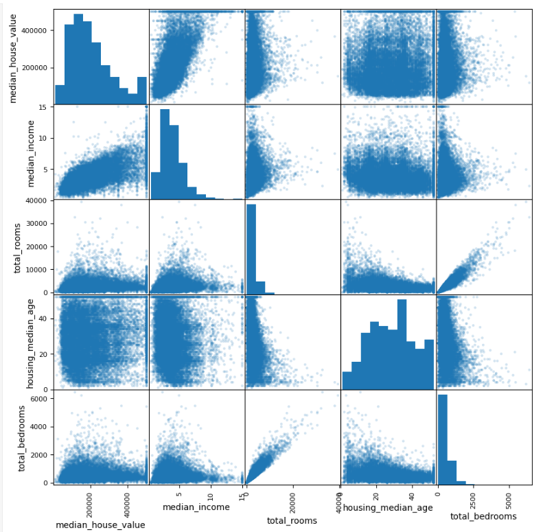
9. 특성 간 상관관계 및 시각화

공분산은 데이터의 관계를 이해하고,
다중공선성은 예측 모델의 성능을 유지하며 해석 가능성을 높이기 위해 중요함.

주요 특성 간의 상관관계를 계산하고 산점도 행렬로 시각화하여 관계를 탐구함.

attributes = ["median_house_value", "median_income", "total_rooms", "housing_median_age", "total_bedrooms"]
corr_matrix = housing[attributes].corr()

fig = scatter_matrix(housing[attributes], figsize=(10, 10), alpha=0.2)

plt.show()

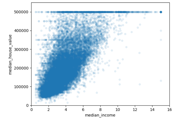
10. 특정 특성 간의 관계 시각화

중간 소득과 주택 가치 간의 관계를 산점도로 분석하여 상관성을 탐구함.

housing.plot(kind="scatter", x="median_income", y="median_house_value", alpha=0.1)

plt.axis([0, 16, 0, 550000])

plt.show()

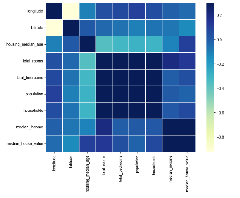
11. 상관관계 히트맵 생성

상관계수를 히트맵으로 표현하여 특성 간의 강한 양/음의 상관관계를 시각적으로 확인함.

import seaborn as sns

corr = housing[housing.columns[:9]].corr()

f, ax = plt.subplots(figsize=(10, 7))

with sns.axes_style("white"):
sns.heatmap(corr, vmax=0.3, cmap="YlGnBu", square=True, linewidths=0.3)
plt.show()

12. 파생변수 생성

새로운 파생변수를 생성하여 데이터를 더욱 세밀하게 분석할 준비를 함.

housing["rooms_per_household"] = housing["total_rooms"] / housing["households"]
housing["bedrooms_per_room"] = housing["total_bedrooms"] / housing["total_rooms"]
housing["population_per_household"] = housing["population"] / housing["households"]

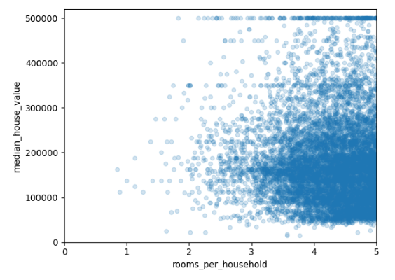
13. 파생변수와 주택 가격 간 관계 분석

가구당 방 수와 주택 가치 간의 관계를 시각적으로 탐구함.

housing.plot(kind="scatter", x="rooms_per_household", y="median_house_value", alpha=0.2)

plt.axis([0, 5, 0, 520000])

plt.show()

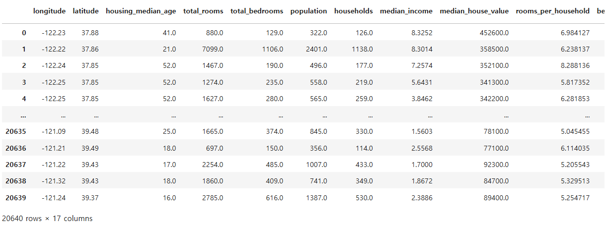
14. 원-핫 인코딩

범주형 데이터를 원-핫 인코딩하여 머신러닝 알고리즘에 적합한 형식으로 변환함.
변환된 데이터프레임을 출력하여 새로운 형식과 특성 확인.

df = pd.get_dummies(data=housing, columns=["ocean_proximity"])

15. 결측치 처리

결측치 처리: 상황에 따라 결측치를 대처하는 값이 다름
결측값을 어떻게 처리할 것인가

from sklearn.impute import SimpleImputer

#중앙값으로 결측치 처리
imputer = SimpleImputer(strategy="median")

housing_num = housing.drop('ocean_proximity', axis=1)

imputer.fit(df)
X = imputer.transform(df)
housing_tr = pd.DataFrame(X, columns=df.columns)
housing_tr.tail()

16. 데이터 분리

주택 가격(median_house_value)을 레이블로 분리하고, 학습 데이터에서 제거함.

housing_labels = housing_tr["median_house_value"].copy() # 레이블로 사용

housing_tr.drop("median_house_value", axis=1, inplace=True) # 레이블 삭제

from sklearn.preprocessing import StandardScaler

scaler = StandardScaler()

18. 데이터 정규화

데이터를 표준 정규화하여 평균 0, 분산 1로 스케일링함.

from sklearn.preprocessing import StandardScaler

scaler = StandardScaler()
scaled_df = scaler.fit_transform(housing_tr)
scaled_df.shape

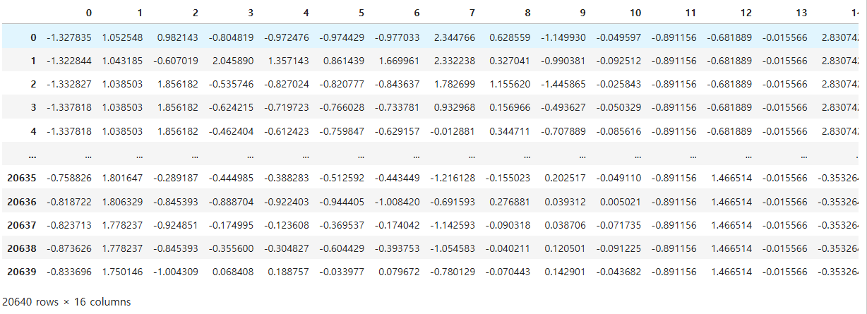
(20640, 16)

19. 정규화된 데이터 확인

정규화된 데이터를 확인하여 변환 결과를 검토함.

scaled_df

pd.DataFrame(scaled_df)

20. 데이터 분리

데이터를 학습용(80%)과 테스트용(20%)으로 분리하여 모델 검증을 준비함.

from sklearn.model_selection import train_test_split

X_train, X_test, y_train, y_test = train_test_split(
scaled_df, housing_labels, test_size=0.2, random_state=42
)

(16512, 16) (4128, 16)

21. 선형 회귀 모델 학습

선형 회귀 모델을 사용해 학습 데이터를 기반으로 주택 가격을 예측하는 모델을 생성함.

from sklearn.linear_model import LinearRegression

lin_reg = LinearRegression(n_jobs=-1)
lin_reg.fit(X_train, y_train)

LinearRegression(n_jobs=-1)
In a Jupyter environment, please rerun this cell to show the HTML representation or trust the notebook.
On GitHub, the HTML representation is unable to render, please try loading this page with nbviewer.org.

22. 선형 회귀 모델 평가

테스트 데이터로 예측값을 생성하고 평균 제곱 오차(RMSE)를 계산하여 모델 성능을 평가함.

from sklearn.metrics import mean_squared_error

y_pred = lin_reg.predict(X_test)
rms = np.sqrt(mean_squared_error(y_test, y_pred))
print(rms)

69129.02662101173

23. 결정 트리 모델 학습 및 평가

결정 트리 모델을 사용해 학습하고, 테스트 데이터로 평가하여 RMSE를 확인함.

from sklearn.tree import DecisionTreeRegressor

tree_reg = DecisionTreeRegressor()
tree_reg.fit(X_train, y_train)

y_pred = tree_reg.predict(X_test)
rms = np.sqrt(mean_squared_error(y_test, y_pred))
print(rms)

69903.69210288586

24. 랜덤 포레스트 모델 학습 및 평가

랜덤 포레스트 모델로 학습 및 평가를 진행하여 가장 낮은 RMSE를 탐색함.

from sklearn.ensemble import RandomForestRegressor

forest_reg = RandomForestRegressor()
forest_reg.fit(X_train, y_train)

y_pred = forest_reg.predict(X_test)
rms = np.sqrt(mean_squared_error(y_test, y_pred))
print(rms)

49804.81319048334

서포트 벡터 머신

서포트 벡터 머신 (SVM) 모델 학습 및 평가

SVM 회귀 모델로 데이터를 학습하고, 테스트 데이터로 RMSE를 계산하여 모델 성능을 평가함.

from sklearn.svm import SVR

svm_reg = SVR(kernel="linear")
svm_reg.fit(X_train, y_train)

y_pred = svm_reg.predict(X_test)
rms = np.sqrt(mean_squared_error(y_test, y_pred))
print(rms)

106532.35352547036

랜덤 포레스트의 최적 파라미터 찾기 (Grid Search)

그리드 서치를 사용해 랜덤 포레스트의 최적의 하이퍼파라미터를 탐색함.

from sklearn.model_selection import GridSearchCV

param_grid = [
{"n_estimators": [3, 10, 30], "max_features": [2, 4, 6, 8]},
{"bootstrap": [False], "n_estimators": [3, 10], "max_features": [2, 3, 4]},
]

forest_reg = RandomForestRegressor(random_state=42, n_jobs=-1)

grid_search = GridSearchCV(
forest_reg,
param_grid,
cv=5,
scoring="neg_mean_squared_error",
return_train_score=True,
)
grid_search.fit(X_train, y_train)

GridSearchCV(cv=5, estimator=RandomForestRegressor(n_jobs=-1, random_state=42),
             param_grid=[{'max_features': [2, 4, 6, 8],
                          'n_estimators': [3, 10, 30]},
                         {'bootstrap': [False], 'max_features': [2, 3, 4],
                          'n_estimators': [3, 10]}],
             return_train_score=True, scoring='neg_mean_squared_error')
In a Jupyter environment, please rerun this cell to show the HTML representation or trust the notebook.
On GitHub, the HTML representation is unable to render, please try loading this page with nbviewer.org.

그리드 서치 결과 출력

그리드 서치의 교차 검증 결과를 출력하여 각 파라미터 조합의 RMSE를 확인함.

cvres = gridsearch.cv_results
for mean_score, params in zip(cvres["mean_test_score"], cvres["params"]):
print(np.sqrt(-mean_score), params)

63771.336777432225 {'max_features': 2, 'n_estimators': 3}
54839.67145330755 {'max_features': 2, 'n_estimators': 10}
52771.57076014853 {'max_features': 2, 'n_estimators': 30}
60227.74294726968 {'max_features': 4, 'n_estimators': 3}
52030.3929705949 {'max_features': 4, 'n_estimators': 10}
49974.72379834999 {'max_features': 4, 'n_estimators': 30}
57648.65377635183 {'max_features': 6, 'n_estimators': 3}
51021.059160783894 {'max_features': 6, 'n_estimators': 10}
49393.26223006682 {'max_features': 6, 'n_estimators': 30}
58942.023680153616 {'max_features': 8, 'n_estimators': 3}
51948.28344277779 {'max_features': 8, 'n_estimators': 10}
49958.84411129611 {'max_features': 8, 'n_estimators': 30}
62094.78975341348 {'bootstrap': False, 'max_features': 2, 'n_estimators': 3}
53956.354098990254 {'bootstrap': False, 'max_features': 2, 'n_estimators': 10}
58049.86787130804 {'bootstrap': False, 'max_features': 3, 'n_estimators': 3}
51462.31613344042 {'bootstrap': False, 'max_features': 3, 'n_estimators': 10}
59141.3538483309 {'bootstrap': False, 'max_features': 4, 'n_estimators': 3}
51717.547123878576 {'bootstrap': False, 'max_features': 4, 'n_estimators': 10}

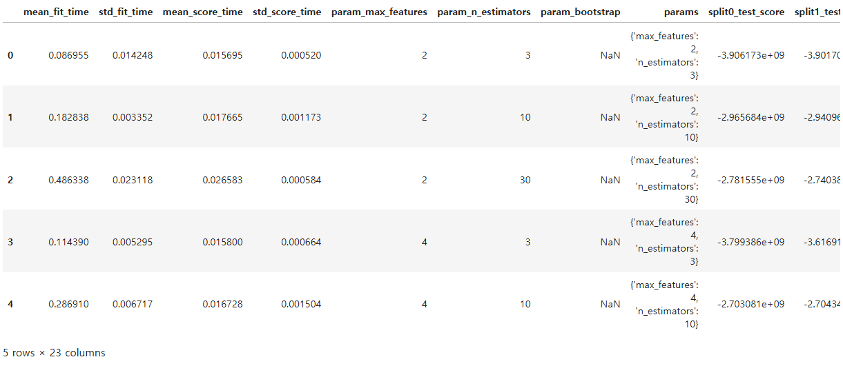
결과 요약 데이터프레임 확인

cv = pd.DataFrame(gridsearch.cv_results)

cv.head()

특성 중요도 시각화

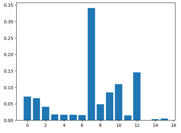
최적 모델에서의 특성 중요도를 시각화하여 각 특성의 기여도를 확인함.

featureimportances = grid_search.best_estimator.featureimportances

plt.bar(range(len(feature_importances)), feature_importances)

plt.show()

랜덤 서치 (Randomized Search)

랜덤 서치를 사용해 랜덤 포레스트 모델의 하이퍼파라미터를 탐색함.

from sklearn.model_selection import RandomizedSearchCV
from scipy.stats import randint

param_distribs = {
"n_estimators": randint(low=1, high=200),
"max_features": randint(low=1, high=8),
}

forest_reg = RandomForestRegressor(random_state=42, n_jobs=-1)
rnd_search = RandomizedSearchCV(
forest_reg,
param_distributions=param_distribs,
n_iter=10,
cv=5,
scoring="neg_mean_squared_error",
random_state=42,
)
rnd_search.fit(X_train, y_train)

RandomizedSearchCV(cv=5,
                   estimator=RandomForestRegressor(n_jobs=-1, random_state=42),
                   param_distributions={'max_features': <scipy.stats._distn_infrastructure.rv_discrete_frozen object at 0x0000024068BB3F90>,
                                        'n_estimators': <scipy.stats._distn_infrastructure.rv_discrete_frozen object at 0x0000024068BC8590>},
                   random_state=42, scoring='neg_mean_squared_error')
In a Jupyter environment, please rerun this cell to show the HTML representation or trust the notebook.
On GitHub, the HTML representation is unable to render, please try loading this page with nbviewer.org.

랜덤 서치 결과 출력

랜덤 서치의 교차 검증 결과를 출력하여 각 파라미터 조합의 RMSE를 확인함.

cvres = rnd_search.cv_results_
for mean_score, params in zip(cvres["mean_test_score"], cvres["params"]):
    print(np.sqrt(-mean_score), params) #양수 처리


cvres = rnd_search.cv_results_
for mean_score, params in zip(cvres["mean_test_score"], cvres["params"]):
    print(np.sqrt(-mean_score), params) #양수 처리
49092.730755569704 {'max_features': 7, 'n_estimators': 180}
51593.829302281534 {'max_features': 5, 'n_estimators': 15}
50104.28738111979 {'max_features': 3, 'n_estimators': 72}
50577.696825486964 {'max_features': 5, 'n_estimators': 21}
49181.72260190157 {'max_features': 7, 'n_estimators': 122}
50132.08012104677 {'max_features': 3, 'n_estimators': 75}
50005.87036054742 {'max_features': 3, 'n_estimators': 88}
49441.74858087694 {'max_features': 5, 'n_estimators': 100}
49890.50937887523 {'max_features': 3, 'n_estimators': 150}
64746.67002116126 {'max_features': 5, 'n_estimators': 2}

최적 모델 파라미터 확인

rndsearch.best_params

랜덤 서치에서 선택된 최적의 하이퍼파라미터를 출력함.

최종 모델 평가

다음 추가된 코드들에 대해 핵심 내용을 요약하여 정리했음:

25. 서포트 벡터 머신 (SVM) 모델 학습 및 평가

SVM 회귀 모델로 데이터를 학습하고, 테스트 데이터로 RMSE를 계산하여 모델 성능을 평가함.

from sklearn.svm import SVR

svm_reg = SVR(kernel="linear")
svm_reg.fit(X_train, y_train)

y_pred = svm_reg.predict(X_test)
rms = np.sqrt(mean_squared_error(y_test, y_pred))

print(rms)

26. 랜덤 포레스트의 최적 파라미터 찾기 (Grid Search)

그리드 서치를 사용해 랜덤 포레스트의 최적의 하이퍼파라미터를 탐색함.

from sklearn.model_selection import GridSearchCV

param_grid = [
{"n_estimators": [3, 10, 30], "max_features": [2, 4, 6, 8]},
{"bootstrap": [False], "n_estimators": [3, 10], "max_features": [2, 3, 4]},
]

forest_reg = RandomForestRegressor(random_state=42, n_jobs=-1)

grid_search = GridSearchCV(
forest_reg,
param_grid,
cv=5,
scoring="neg_mean_squared_error",
return_train_score=True,
)
grid_search.fit(X_train, y_train)

27. 그리드 서치 결과 출력

그리드 서치의 교차 검증 결과를 출력하여 각 파라미터 조합의 RMSE를 확인함.

cvres = gridsearch.cv_results
for mean_score, params in zip(cvres["mean_test_score"], cvres["params"]):
print(np.sqrt(-mean_score), params)

28. 결과 요약 데이터프레임 확인

그리드 서치의 교차 검증 결과를 데이터프레임으로 확인하여 세부 정보를 분석함.

cv = pd.DataFrame(gridsearch.cv_results)
cv.head()

29. 특성 중요도 시각화

최적 모델에서의 특성 중요도를 시각화하여 각 특성의 기여도를 확인함.

feature_importances =

gridsearch.best_estimator.featureimportances

plt.bar(range(len(feature_importances)), feature_importances)

plt.show()

30. 랜덤 서치 (Randomized Search)

랜덤 서치를 사용해 랜덤 포레스트 모델의 하이퍼파라미터를 탐색함.

from sklearn.model_selection import RandomizedSearchCV
from scipy.stats import randint

param_distribs = {
"n_estimators": randint(low=1, high=200),
"max_features": randint(low=1, high=8),
}

31. 랜덤 서치 결과 출력

랜덤 서치의 교차 검증 결과를 출력하여 각 파라미터 조합의 RMSE를 확인함.

cvres = rndsearch.cv_results
for mean_score, params in zip(cvres["mean_test_score"], cvres["params"]):
print(np.sqrt(-mean_score), params)

49092.730755569704 {'max_features': 7, 'n_estimators': 180}
51593.829302281534 {'max_features': 5, 'n_estimators': 15}
50104.28738111979 {'max_features': 3, 'n_estimators': 72}
50577.696825486964 {'max_features': 5, 'n_estimators': 21}
49181.72260190157 {'max_features': 7, 'n_estimators': 122}
50132.08012104677 {'max_features': 3, 'n_estimators': 75}
50005.87036054742 {'max_features': 3, 'n_estimators': 88}
49441.74858087694 {'max_features': 5, 'n_estimators': 100}
49890.50937887523 {'max_features': 3, 'n_estimators': 150}
64746.67002116126 {'max_features': 5, 'n_estimators': 2}

32. 최적 모델 파라미터 확인

랜덤 서치에서 선택된 최적의 하이퍼파라미터를 출력함.

rndsearch.best_params

{'max_features': 7, 'n_estimators': 180}

33. 최종 모델 평가

랜덤 서치로 선택된 최적 모델을 사용해 테스트 데이터의 RMSE를 계산하여 최종 성능을 평가함.

finalmodel = rnd_search.best_estimator

y_pred = final_model.predict(X_test)

rms = np.sqrt(mean_squared_error(y_test, y_pred))

print(rms)

용어 정리

히트맵: 변수 간 상관관계를 색상으로 시각화한 차트임.

파생변수: 기존 데이터를 기반으로 새롭게 생성된 변수임.

원핫인코딩: 범주형 변수를 이진 변수로 변환하는 기법임.

데이터 정규화: 데이터를 일정한 범위로 변환하여 비교 가능하게 만드는 기법임.

선형회귀: 독립 변수와 종속 변수 간의 관계를 직선으로 모델링하는 통계적 방법임.

결정트리모델: 데이터를 분할하여 예측을 수행하는 트리 구조 기반 모델임.

RMSE (Root Mean Squared Error): 예측값과 실제값 간의 차이를 제곱하여
평균을 낸 후, 그 값의 제곱근을 구한 오차 측정값임.

랜덤포레스트: 여러 개의 결정 트리를 결합하여 예측 성능을 향상시키는 앙상블 모델임.

서포트벡터머신 (SVM): 고차원 공간에서 분류 및 회귀를 수행하는 지도 학습 모델임.

파라미터: 모델이 학습되는 과정에서 최적화되는 값들임.

그리드 서치: 주어진 하이퍼파라미터의 모든 조합을 테스트하여 최적의 모델을 찾는 기법임.

랜덤 서치: 하이퍼파라미터의 범위 내에서 무작위로 조합을 선택하여 최적 모델을 찾는 기법임.

교차 검증: 데이터를 여러 부분으로 나누어 모델을 평가하는 기법으로, 과적합을 방지하는 데 유용함.

이현지

관심분야: 추천시스템, 자연어처리, 머신러닝, 딥러닝

이전 포스트

[R] 통계적 분석 기법(t-test)

다음 포스트

[머신러닝] 의사결정나무, 서포트벡터머신

R/머신러닝/딥러닝

1. 라이브러리 임포트 및 설정

2. 데이터 다운로드 함수 정의 및 실행

깃허브를 통한 데이터 다운

3. 데이터 로드 및 미리보기

6. 데이터 통계 요약

7. 데이터분포 확인

8. 위경도 기반 지리정보 시각화

9. 특성 간 상관관계 및 시각화

10. 특정 특성 간의 관계 시각화

11. 상관관계 히트맵 생성

12. 파생변수 생성

13. 파생변수와 주택 가격 간 관계 분석

14. 원-핫 인코딩

15. 결측치 처리

16. 데이터 분리

18. 데이터 정규화

19. 정규화된 데이터 확인

20. 데이터 분리

21. 선형 회귀 모델 학습

22. 선형 회귀 모델 평가

23. 결정 트리 모델 학습 및 평가

24. 랜덤 포레스트 모델 학습 및 평가

서포트 벡터 머신

서포트 벡터 머신 (SVM) 모델 학습 및 평가

랜덤 포레스트의 최적 파라미터 찾기 (Grid Search)

그리드 서치 결과 출력

결과 요약 데이터프레임 확인

특성 중요도 시각화

랜덤 서치 (Randomized Search)

랜덤 서치 결과 출력

최적 모델 파라미터 확인

최종 모델 평가

25. 서포트 벡터 머신 (SVM) 모델 학습 및 평가

26. 랜덤 포레스트의 최적 파라미터 찾기 (Grid Search)

27. 그리드 서치 결과 출력

28. 결과 요약 데이터프레임 확인

29. 특성 중요도 시각화

30. 랜덤 서치 (Randomized Search)

31. 랜덤 서치 결과 출력

32. 최적 모델 파라미터 확인

33. 최종 모델 평가

용어 정리

[R] 통계적 분석 기법(t-test)

[R] Rstudio(R스튜디오) 수동 업데이트 방법

0개의 댓글