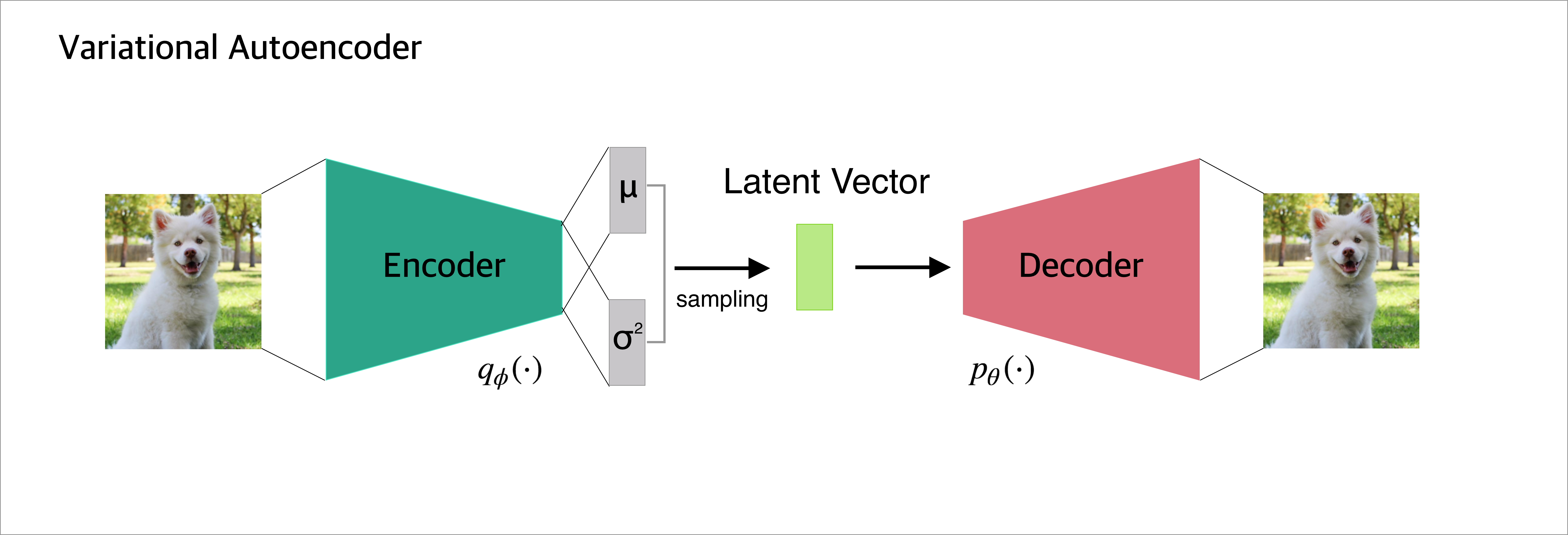
VAE 구조

이 구조에서 input 그림이 있을 때 어떤 의미를 가진 구조를 거쳐 output이 나오게 되는지 3 단계로 나누어 살펴볼 것이다.

⏳ 단계별 과정
1. input: x –> 𝑞∅ (𝑥)–> 𝜇𝑖,𝜎𝑖
2. 𝜇𝑖, 𝜎𝑖, 𝜖𝑖 –> 𝑧𝑖
3. 𝑧𝑖 –> 𝑔𝜃 (𝑧𝑖) –> 𝑝_𝑖 : output

1. Encoder

input: x –> 𝑞∅ (𝑥)–> 𝜇𝑖,𝜎_𝑖

• Input shape(x) : (28,28,1)
• 𝑞_∅ (𝑥) 는 encoder 함수인데, x가 주어졌을때(given) z값의 분포의 평균과 분산을 아웃풋으로 내는 함수이다.

  Encoder 함수의 output은 latent variable의 분포의 𝜇 와 𝜎 를 내고, 이 output값을 표현하는 확률밀도함수를 생각해볼 수 있다.

# VAE encoder network
img_shape = (28,28, 1)
batch_size = 16
latent_dim = 2

encoder_input = keras.Input(shape = img_shape, name='Encoder_Input')
x = encoder_input

x = layers.Conv2D(32, 3, padding = 'same', activation='relu')(x)
x = layers.Conv2D(64, 3, padding = 'same', activation='relu', strides=(2, 2))(x)
x = layers.Conv2D(64, 3, padding = 'same', activation='relu')(x)
x = layers.Conv2D(64, 3, padding = 'same', activation='relu')(x)

# return tuple of integers of shape of x
# (14, 14, 64)
shape_before_flattening = K.int_shape(x)[1:]

x = layers.Flatten()(x) # (None, 12544)
x = layers.Dense(32, activation='relu')(x) # (None, 32)

z_mean = layers.Dense(latent_dim)(x)
z_log_var = layers.Dense(latent_dim)(x)

2. Reparameterization Trick (Sampling)

𝜇𝑖, 𝜎𝑖, 𝜖𝑖 –> 𝑧𝑖

sampling 과정이 없다면 encoder 결과에서 나온 값에 대한 decoder역시 한 값만 가지게 된다. 따라서 우리는 필연적으로 그 데이터의 확률분포와 같은 분포에서 하나를 뽑는 sampling을 해야한다. 하지만 그냥 sampling 한다면 sampling 한 값들을 backpropagation 할 수 없다.이를 해결하기 위해 reparmeterization trick을 사용한다고 한다.

정규분포에서 z1를 샘플링하는 것이나, 입실론을 정규분포(자세히는 N(0,1))에서 샘플링하고 그 값을 분산과 곱하고 평균을 더해 z2를 만들거나 두 z1,z2 는 같은 분포를 가진다고 한다.

그래서 코드에서 epsilon을 먼저 정규분포에서 random하게 뽑고, 그 epsilon을 exp(z_log_var)과 곱하고 z_mean을 더한다. 그렇게 형성된 값이 z가 된다.

latent variable에서 sample된 z라는 value (= decoder input)가 만들어진다.

# latent_space_sampling function

def sampling(args):
  z_mean, z_log_var = args
  # 정규분포로부터의 난수값을 반환
  epsilon = K.random_normal(shape=(K.shape(z_mean)[0], latent_dim), mean=0., stddev=1.)
  return z_mean + K.exp(z_log_var) * epsilon

z = layers.Lambda(sampling)([z_mean, z_log_var])

3. Decoder

𝑧𝑖 –> 𝑔𝜃 (𝑧𝑖) –> 𝑝𝑖 : output

z 값을 g 함수(decoder)에 넣고 deconv(Conv2DTranspose)를 해 원래 이미지 사이즈의 아웃풋 z_decoded가 나오게 된다. 이때 p_data(x)의 분포를 Bernoulli 로 가정했으므로 output 값은 0~1 사이 값을 가져야하고, 이를 위해 마지막 activatino function이 sigmoid로 설정되는 것이다.

VAE decoder network

latent space의 포인트를 이미지로 맵핑

decoder_input = layers.Input(K.int_shape(z)[1:]) # 잠재벡터의 차원(latent_dim) 과 같다
x = layers.Dense(np.prod(shape_before_flattening), activation = 'relu')(decoder_input) # np.prod(): 각 배열 요소를 곱함
x = layers.Reshape(shape_before_flattening)(x)
x = layers.Conv2DTranspose(32, 3, padding='same', activation='relu', strides=(2,2))(x)
x = layers.Conv2D(1, 3, padding='same', activation='sigmoid')(x)

decoder_output = x
decoder = Model(inputs = decoder_input, outputs = decoder_output, name="Decoder")
z_decoded = decoder(z)

VAE 학습

Loss Function 이해

Loss 는 크게 총 2가지 부분이 있다.

• Reconstruction Loss(code에서는 xent_loss)
• Regularization Loss(code에서는 kl_loss)

Reconstruction Loss : X 와 New X와의 관계

디코더 부분의 pdf는 Bernoulli 분포를 따른다고 가정했으므로 그 둘간의 cross entropy를 구한다.

Regularization Loss : X의 분포와 근사한 분포의 차이

X가 원래 가지는 분포와 동일한 분포를 가지게 학습하게 하기위해 true 분포를 approximate 한 함수의 분포에 대한 loss term이 Regularization Loss다. 이때 loss는 true pdf 와 approximated pdf간의 D_kl(두 확률분포의 차이(거리))을 계산한다.

# Custom layer used to compute the VAE loss

class CustomVariationalLayer(keras.layers.Layer):

  def vae_loss(self, x, z_decoded):
    x = K.flatten(x)
    print(K.shape(x))
    z_decoded = K.flatten(z_decoded)
    print(K.shape(z_decoded))
    xent_loss = keras.metrics.binary_crossentropy(x, z_decoded)
    kl_loss = -5e-4*K.mean(1+z_log_var-K.square(z_mean)-K.exp(z_log_var), axis=-1)
    return K.mean(xent_loss + kl_loss)

  def call(self, inputs):
    x = inputs[0]
    z_decoded = inputs[1]
    loss = self.vae_loss(x,z_decoded)
    self.add_loss(loss, inputs=inputs)
    return x

y = CustomVariationalLayer()([encoder_input, z_decoded]) # check

# Training the VAE

vae = Model(encoder_input, y)
vae.compile(optimizer='rmsprop',loss=None) # Model.compile(loptimizer, loss, metrics)
vae.summary()

Reference
[https://github.com/Taeu/FirstYear_RealWorld/blob/master/GoogleStudy/Keras_week8_2/8.4%20VAE.ipynb]