Spectral Density

김당찬·2023년 1월 12일

Spectral Representation Theorem

시계열 자료는 $\{x_{t}: t=1\ldots T\}$ 형태로 discrete하게 주어진다. 반면, 파동함수(cosine, sine function)를 이용해 시계열 자료를 근사하는 방법이 있는데, 이러한 형태로 주어진 자료를 spectral 하다고 한다. Spectral Representation Theorem은, 임의의 discrete한 시계열 자료가 stationary하기만 하면 spectral form으로 근사할 수 있음을 의미한다. 이와 관련해 다음 두 정리가 성립한다.

Theorem 1

함수 $\gamma(h) : h=0,\pm1,\pm2,\ldots$ 가 non-negative definite일 필요충분조건은

\gamma(h) = \int^{\frac{1}{2}}_{-\frac{1}{2}}\exp(2\pi iwh)dF(w)

로 주어지며 함수 $F$ 가 right-continuous이며, 적분구간 내 유계이고 조건 $F(-\frac{1}{2})=0, F(\frac{1}{2})=0$ 에 의해 유일하게 결정된다는 것이다.

이때 함수 $\gamma(h)$ 는 시계열 자료의 autocovariance function을 생각하면 되며, 새로이 주어지는 함수 $F$ 는 spectral density function 이라고 정의한다. 또한, 함수가 non-negative definite하다는 것은 다음 조건을 의미한다.

\gamma_x(h)=E[x_{t+h}x_{t}^{*}]\text{ 로 주어질 때 } E|\sum_{s=1}^{n}a_{s}^{*}x_{s}|^{2}\geq 0\;\;for\;\;\forall a_{t}\in\mathbb C

Theorem 2

시계열 $\{x_t\}$ 가 stationary하고 평균이 0이며 spectral density가 앞선 정리 1과 같이 $F(w)$ 로 주어진다고 하자. 그러면 complex-valued stochastic process $Z(w)$ 가 $w\in[- \frac{1}{2},\frac{1}{2}]$ 에 존재하여 stationary한 uncorrelated increments를 갖고, 다음과 같이 주어진다.

x_{t}= \int_{- \frac{1}{2}}^{\frac{1}{2}}\exp(-2\pi itw) dZ(w)

where for $- \frac{1}{2}\leq w_{1}\leq w_{2}\leq \frac{1}{2}$ , $Var(Z(w_{2})-Z(w_{1})) = F(w_{2})-F(w_{1})$

Spectral Density Function

앞선 정리로 주어진 spectral density를 일반적인 확률론에서 probability density에 유추할 수 있다. 개별 확률밀도함수에 대해 적률생성함수나 특성함수가 유일하게 결정되는 것과 유사하게, 각 시계열의 spectral density에 대해서도 특성함수에 대응하는 함수가 존재하는데, 그것이 바로 autocovariance function이다. 즉, 다음과 같은 정리가 성립한다.

Property

Stationary process의 autocovariance function $\gamma(h)$ 에 대해 $\sum_{h=-\infty}^{\infty}|\gamma(h)|<\infty$ 를 만족하면 spectral density function과 다음 표현관계가 성립한다.

\gamma(h)=\int_{- \frac{1}{2}}^{\frac{1}{2}}\exp(2\pi iwh)f(w)dw\Leftrightarrow f(w)=\sum_{h=-\infty}^{\infty} \gamma(h)\exp(-2\pi iwh)

이때, spectral density

f(w) = \sum\gamma(h)\exp(-2\pi iwh) = \sum\gamma(h)(\cos(2\pi wh)-i\sin(2\pi wh))

로부터,

f(w)=f(-w), \;\;f(w) = f(1-w)

이므로 spectral density는 주기가 1인 even function이다. 따라서 일반적으로 plot은 $0\leq w\leq \frac{1}{2}$ 인 범위에서 그린다.

Discrete Fourier Tranformation(DFT)

시계열 $\{x_t\}$ 에 대한 discrete fourier transformation은 다음과 같이 주어진다.

d(w_{j}) = \frac{1}{\sqrt n}\sum_{t=1}^{n}x_{t}\exp (-2\pi iw_{j}t)

이때 $w_{j}$ 는 $w_{j}=\frac{j}{n}, j=0,\cdots ,n-1$ 으로 주어지는데, 이 값들을 Fourier frequency 혹은 Fundamental frequency라고 한다. DFT는 n이 매우 큰 합성수인 경우 Fast Fourier Transformation(FFT) 알고리즘으로 계산할 수 있다.

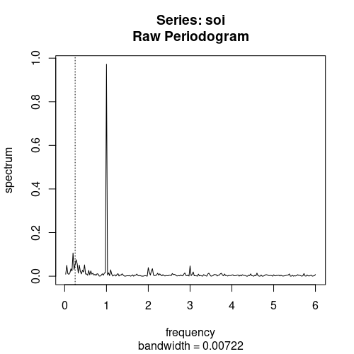
Periodogram

주기도(periodogram)은 임의의 시계열에 대한 DFT를 바탕으로, 각 시계열의 spectral density에 포함된 개별 주기함수가 어떠한 주기(혹은 진동수, frequency)를 포함하는지 나타내는 plot이다. DFT의 각 fundamental frequency들에 대한 value를 나타내며, 해당 fundamental frequency의 periodogram 값이 클 수록 해당 진동수가 포함되어있음을 의미한다. Periodogram은 다음과 같이 주어진다.