
📊 DL 분류모델
📌 DL 분류 특징 - 기울기 소실 문제
- 특징
- 분류 모델에서 Layer 개수가 많아지는 것이 관습적이다.
- Layer 개수가 많아질수록 기울기 소실 문제가 발생한다.
- 기울기 소실 문제
- 데이터가 Layer를 지나갈수록 기울기와 편향값이 점점 소실되는 문제이다.
→ [ 이를 해결하기 위해 은닉층의 활성화함수로 ReLU를 사용한다. ]
📊 DL 분류모델 실습
📌 DL 분류 실습
1. 라이브러리 Import
# 기본 라이브러리
import pandas as pd
import numpy as np
import matplotlib.pyplot as plt
import seaborn as sns

# 학습, 테스트 데이터 분리
from sklearn.model_selection import train_test_split

# 딥러닝 네트워크
from keras.models import Model
from keras.layers import Input, Dense, Concatenate
from keras.optimizers import Adam

# 조기종료, 체크포인트
from keras.callbacks import EarlyStopping, ModelCheckpoint

# 분류모델 성능 평가 지표
from sklearn.metrics import accuracy_score
2. 데이터 준비
data = pd.read_csv('../testdata/wine.csv', header=None)
print(data.head(2))
#     0     1    2    3      4     5     6       7     8     9    10  11  12
# 0  7.4  0.70  0.0  1.9  0.076  11.0  34.0  0.9978  3.51  0.56  9.4   5   1
# 1  7.8  0.88  0.0  2.6  0.098  25.0  67.0  0.9968  3.20  0.68  9.8   5   1
3. 데이터 정보 및 결측값 확인
print(data.info())
# RangeIndex: 6497 entries, 0 to 6496
#  #   Column  Non-Null Count  Dtype
# ---  ------  --------------  -----
#  0   0       6497 non-null   float64
#  1   1       6497 non-null   float64
#  2   2       6497 non-null   float64
#  3   3       6497 non-null   float64
#  4   4       6497 non-null   float64
#  5   5       6497 non-null   float64
#  6   6       6497 non-null   float64
#  7   7       6497 non-null   float64
#  8   8       6497 non-null   float64
#  9   9       6497 non-null   float64
#  10  10      6497 non-null   float64
#  11  11      6497 non-null   int64
#  12  12      6497 non-null   int64
# -> 결측값은 존재하지 않음
4. feature, label 분리
feature = data.iloc[:, :-1]
label = data.iloc[:, -1]
5. 학습, 테스트 데이터 분리
x_train, x_test, y_train, y_test = train_test_split(feature, label, test_size=0.3, shuffle=True, stratify=label, random_state=1)
print(x_train.shape, x_test.shape, y_train.shape, y_test.shape)
# (4547, 12) (1950, 12) (4547,) (1950,)

x_train, x_valid, y_train, y_valid = train_test_split(x_train, y_train, test_size=0.2, shuffle=True, stratify=y_train, random_state=1)
print(x_train.shape, x_valid.shape, y_train.shape, y_valid.shape)
# (3637, 12) (910, 12) (3637,) (910,)
6. Functional API 모델 구축
inputs = Input(shape=(12,))
net1 = Dense(units=32, activation='relu')(inputs)
net2 = Dense(units=16, activation='relu')(net1)
concat1 = Concatenate()([inputs, net2])
net3 = Dense(units=8, activation='relu')(concat1)
net4 = Dense(units=4, activation='relu')(net3)
concat2 = Concatenate()([concat1, net4])
net5 = Dense(units=2, activation='relu')(concat2)
outputs = Dense(units=1, activation='sigmoid')(net5)

model = Model(inputs, outputs)
7. 모델 학습 최적화 설정
model.compile(optimizer=Adam(learning_rate=0.001), loss='binary_crossentropy', metrics=['accuracy'])
8. EarlyStopping, ModelCheckpoint 설정
[ ModelCheckpoint 속성 ]
- monitor 속성 : 중간 저장하기 위한 성능 평가 지표 지정
- filepath 속성 : 중간 저장할 모델 파일 위치 지정
- verbose 속성 : 중간 저장 시, 출력 여부 지정
- save_best_only 속성 : 중간 저장 시, 성능이 가장 좋은 시점의 모델로 저장할지 여부 지정es = EarlyStopping( monitor='val_loss', patience=10 ) cp = ModelCheckpoint( monitor='val_loss', filepath='save_model.hdf5', verbose=0, save_best_only=True )
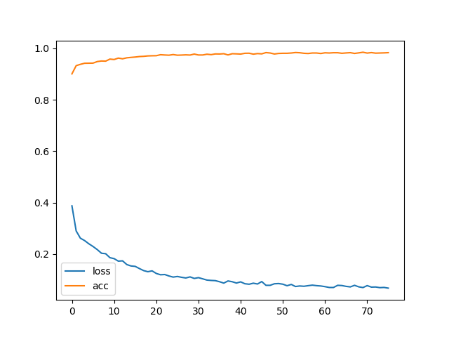
9. 모델 학습
history = model.fit(
    x=x_train,
    y=y_train,
    batch_size=32,
    epochs=500,
    validation_data=(x_valid, y_valid),
    callbacks=[es, cp],
    verbose=1
)
plt.plot(history.history['loss'], label='loss')
plt.plot(history.history['accuracy'], label='acc')
plt.legend()
plt.show()
10. 모델 평가
loss, acc = model.evaluate(
    x=x_test,
    y=y_test,
    batch_size=32,
    verbose=0
)
print('loss : ', loss)
print('acc : ', acc)
# loss :  0.05753648281097412
# acc :  0.9851282238960266
11. 모델 예측값, 실제값 비교
y_pred = model.predict(x=x_test).flatten()
y_pred = [1 if pred > 0.5 else 0 for pred in y_pred]
print('예측값 : ', y_pred[:4])
print('실제값 : ', np.array(y_test)[:4])
# 예측값 :  [1, 0, 0, 0]
# 실제값 :  [1 0 0 0]
12. 분류모델 성능 평가 - 정확도
acc = accuracy_score(y_test, y_pred)
print('정확도 : ', acc)
# 정확도 :  0.9851282051282051

데이터 사이언티스트를 목표로 하는 개발자