📊 XGBoost

---

📌 XGBoost란?

• 정의
  - 앙상블 기법 중 부스팅(boosting) 방식을 사용하는 모델
  - 직렬 처리

---

📌 XGBoost 설치

• 설치 방법
  1) anaconda prompt
  2) pip install xgboost

---

📌 XGBoost 계량종 - lightgbm 설치

• 설치 방법
  1) anaconda prompt
  2) pip install lightgbm

---

📊 XGBoost 실습

---

📌 XGBoost 문제1

1. 라이브러리 Import

import pandas as pd
import numpy as np
import matplotlib.pyplot as plt
import seaborn as sns
from sklearn.preprocessing import LabelEncoder
from sklearn.model_selection import train_test_split

# XGBoost 분류 모델
from xgboost import XGBClassifier

# 분류 모델 성능 평가 지표
from sklearn.metrics import accuracy_score, classification_report

# 앙상블 모델의 특성(feature) 중요도 추출 모듈
from xgboost import plot_importance

---

2. 데이터 준비

data = pd.read_csv('../testdata/glass.csv')
print(data.head(3))
#         RI     Na    Mg    Al     Si     K    Ca   Ba   Fe  Type
# 0  1.52101  13.64  4.49  1.10  71.78  0.06  8.75  0.0  0.0     1
# 1  1.51761  13.89  3.60  1.36  72.73  0.48  7.83  0.0  0.0     1
# 2  1.51618  13.53  3.55  1.54  72.99  0.39  7.78  0.0  0.0     1

---

3. 결측치 확인

print(data.info())
# RangeIndex: 214 entries, 0 to 213
#  #   Column  Non-Null Count  Dtype  
# ---  ------  --------------  -----  
#  0   RI      214 non-null    float64
#  1   Na      214 non-null    float64
#  2   Mg      214 non-null    float64
#  3   Al      214 non-null    float64
#  4   Si      214 non-null    float64
#  5   K       214 non-null    float64
#  6   Ca      214 non-null    float64
#  7   Ba      214 non-null    float64
#  8   Fe      214 non-null    float64
#  9   Type    214 non-null    int64  

print(data.isnull().sum())
# RI      0
# Na      0
# Mg      0
# Al      0
# Si      0
# K       0
# Ca      0
# Ba      0
# Fe      0
# Type    0
# 결측치 없음

---

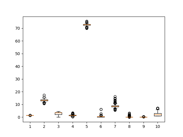
4. 이상치 확인

pd.set_option('display.max_columns', None)
print(data.describe())
#                RI          Na          Mg          Al          Si           K  \
# count  214.000000  214.000000  214.000000  214.000000  214.000000  214.000000   
# mean     1.518365   13.407850    2.684533    1.444907   72.650935    0.497056   
# std      0.003037    0.816604    1.442408    0.499270    0.774546    0.652192   
# min      1.511150   10.730000    0.000000    0.290000   69.810000    0.000000   
# 25%      1.516522   12.907500    2.115000    1.190000   72.280000    0.122500   
# 50%      1.517680   13.300000    3.480000    1.360000   72.790000    0.555000   
# 75%      1.519157   13.825000    3.600000    1.630000   73.087500    0.610000   
# max      1.533930   17.380000    4.490000    3.500000   75.410000    6.210000   
#
#                Ca          Ba          Fe        Type  
# count  214.000000  214.000000  214.000000  214.000000  
# mean     8.956963    0.175047    0.057009    2.780374  
# std      1.423153    0.497219    0.097439    2.103739  
# min      5.430000    0.000000    0.000000    1.000000  
# 25%      8.240000    0.000000    0.000000    1.000000  
# 50%      8.600000    0.000000    0.000000    2.000000  
# 75%      9.172500    0.000000    0.100000    3.000000  
# max     16.190000    3.150000    0.510000    7.000000  

plt.boxplot(data)
plt.show()
# -> 크게 이상치가 있어 보이지는 않음
# -> 추가로 label encoding할 칼럼도 보이지 않음

---

5. label unique 값 확인

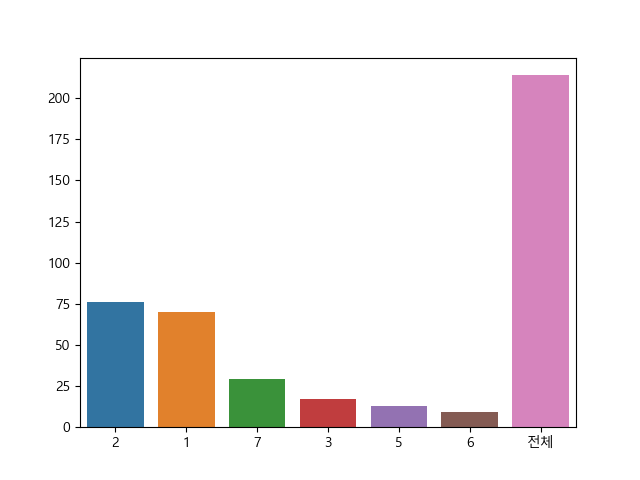
label_tab = data['Type'].value_counts()
label_tab['전체'] = len(data['Type'])
print(label_tab)
# 2      76
# 1      70
# 7      29
# 3      17
# 5      13
# 6       9
# 전체    214
# -> 다중 분류

---

6. label unique 값별 비율 그래프

plt.rc('font', family='malgun gothic')
plt.rcParams['axes.unicode_minus'] = False
sns.barplot(x=label_tab.index, y=label_tab.values)
plt.show()
# -> 2, 1번 label의 빈도가 높음
# -> 학습 시, 편향된 데이터 분포는 성능 저하 원인이 됨

---

7. 학습, 테스트 데이터 분리

features = data.drop(['Type'], axis=1)
label = data['Type']

# 모델 학습 시, label의 unique value는 0부터 시작해야 하므로 Encoding 진행
encoder = LabelEncoder()
label = encoder.fit_transform(label)
label = pd.Series(label, name='Type')

x_train, x_test, y_train, y_test = train_test_split(features, label, test_size=0.3, random_state=10)
print(x_train.shape, x_test.shape, y_train.shape, y_test.shape)
# (149, 4) (65, 4) (149,) (65,)

---

8. 학습, 테스트 label의 비율 분포 비교

train_len = y_train.count()
test_len = y_test.count()
print('학습 데이터 label 비율 분포 :\n', (y_train.value_counts())/train_len)
# 학습 데이터 label 비율 분포 :
# 2    0.395973
# 1    0.302013
# 7    0.140940
# 3    0.067114
# 5    0.060403
# 6    0.033557

print('테스트 데이터 label 비율 분포 :\n', (y_test.value_counts())/test_len)
# 테스트 데이터 label 비율 분포 :
# 1    0.384615
# 2    0.261538
# 7    0.123077
# 3    0.107692
# 5    0.061538
# 6    0.061538
# -> 2, 3, 6번 label의 비율 차이가 발생

---

9. XGBoost 분류 모델

model = XGBClassifier(n_estimators=500, random_state=10)
model.fit(
    x_train, y_train,
    eval_metric='auc',
    eval_set=[[x_train, y_train], [x_test, y_test]],
    early_stopping_rounds=2
)

---

10. 예측값, 실제값 비교

y_pred = model.predict(x_test)
print('예측값 : ', y_pred[:10])
print('실제값 : ', np.array(y_test)[:10])
# 예측값 :  [0 1 1 2 0 1 1 3 0 0]
# 실제값 :  [2 1 1 2 0 1 0 3 0 2]

---

11. 모델 성능 평가 - 정확도

acc = accuracy_score(y_test, y_pred)
print('모델 정확도 : ', acc)
# 모델 정확도 :  0.676923076923077

---

12. 모델 종합 성능 평가 - 정확도, 정밀도, 재현도

report = classification_report(y_test, y_pred)
print(report)
#               precision    recall  f1-score   support
#
#            0       0.71      0.68      0.69        25
#            1       0.56      0.82      0.67        17
#            2       0.50      0.14      0.22         7
#            3       0.80      1.00      0.89         4
#            4       1.00      0.25      0.40         4
#            5       0.88      0.88      0.88         8
#
#     accuracy                           0.68        65
#    macro avg       0.74      0.63      0.62        65
# weighted avg       0.69      0.68      0.65        65

# accuracy : 0.68
# recall : 1번, 3번, 5번 label에 대한 재현도가 높음
# precision : 3번, 4번, 5번 label에 대한 정밀도가 높음

---

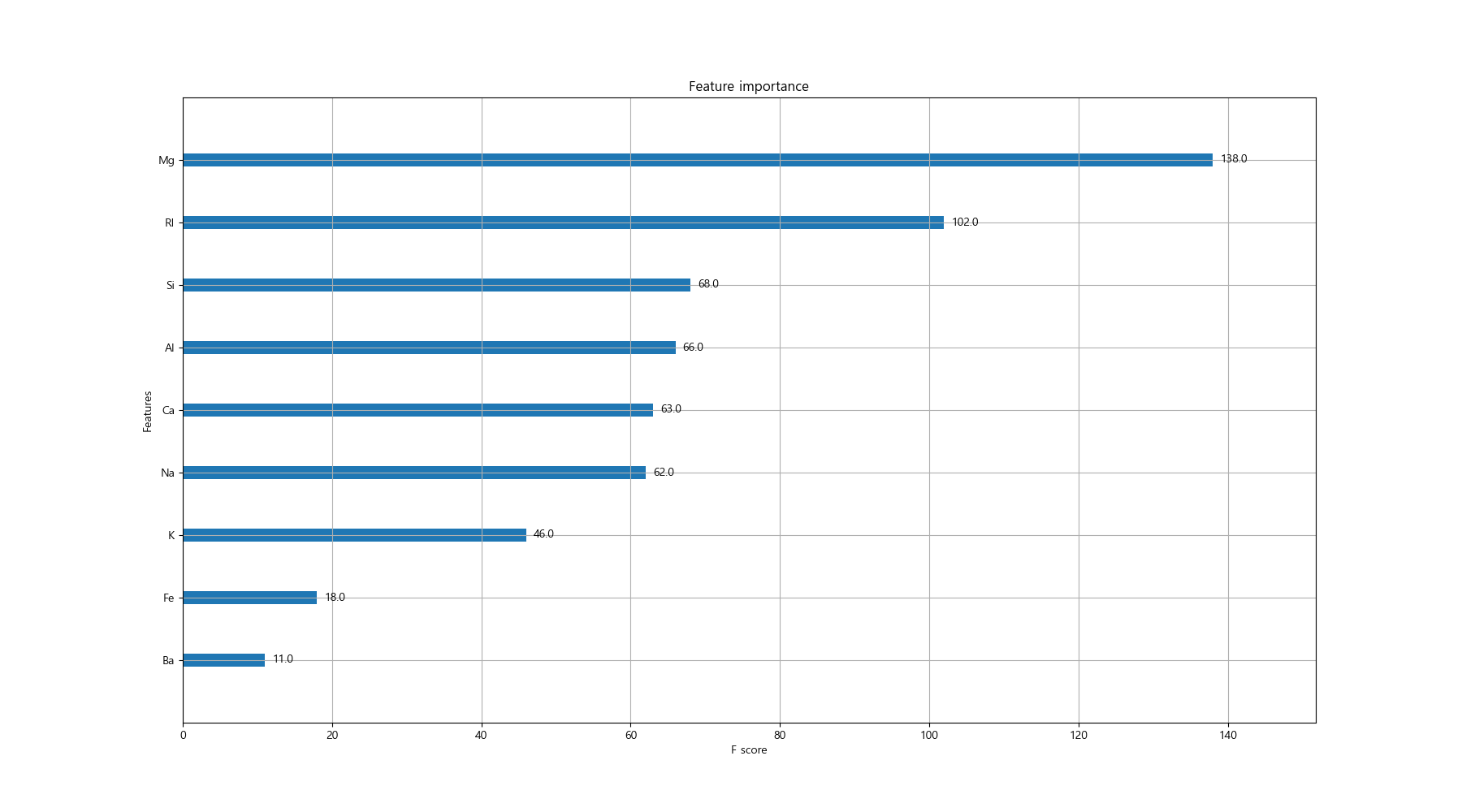
13. 특성 중요도 그리기

fig, ax = plt.subplots(figsize=(18, 10))
plot_importance(model, ax=ax)
plt.show()
# -> K, Fe, Ba 칼럼의 중요도가 상대적으로 낮다.
# -> 위 3개의 칼럼을 빼고 데이터 구성

---