
📊 나이브베이즈 (NaiveBayes)
📌 나이브베이즈란?
- 정의
- 두 확률 변수의 사전확률과 사후확률 사이의 관계를 나타내는 정리
📌 조건부확률
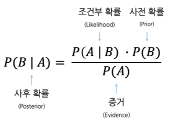
P(B|A) : 사건 A가 일어났을 때, B가 앞서 발생했을 확률 = 사후 확률
P(A) : 사건 A가 일어날 확률
P(B) : 사건 A가 일어나기 전, 사건 B가 일어날 확률 = 사전 확률
P(A|B) : 사건 B가 일어난 후, 사건 A가 발생할 확률 = 조건부 확률
📌 베이즈 정리
- 베이즈 정리
📊 머신러닝 나이브베이즈
📌 ML에서 나이브베이즈란?
- 조건부 확률
⭐ P(Label|Feature) = P(Feature|Label) * P(Label) / P(Feature)
📌 나이브베이즈 실습
- 1. 라이브러리 Import
import pandas as pd
import numpy as np
import matplotlib.pyplot as plt
from sklearn.model_selection import train_test_split, cross_val_score

# 나이브베이즈 분류 모델
from sklearn.naive_bayes import GaussianNB
from sklearn.metrics import accuracy_score, classification_report, roc_curve, auc
- 2. 데이터 준비
data = pd.read_csv('../testdata/weather.csv')
print(data.head(3))
#          Date  MinTemp  MaxTemp  Rainfall  ...  Cloud  Temp  RainToday  RainTomorrow
# 0  2016-11-01      8.0     24.3       0.0  ...      7  23.6         No           Yes
# 1  2016-11-02     14.0     26.9       3.6  ...      3  25.7        Yes           Yes
# 2  2016-11-03     13.7     23.4       3.6  ...      7  20.2        Yes           Yes
- 3. 데이터 정보 확인
print(data.info())
# RangeIndex: 366 entries, 0 to 365
#  #   Column        Non-Null Count  Dtype
# ---  ------        --------------  -----
#  0   Date          366 non-null    object
#  1   MinTemp       366 non-null    float64
#  2   MaxTemp       366 non-null    float64
#  3   Rainfall      366 non-null    float64
#  4   Sunshine      363 non-null    float64
#  5   WindSpeed     366 non-null    int64
#  6   Humidity      366 non-null    int64
#  7   Pressure      366 non-null    float64
#  8   Cloud         366 non-null    int64
#  9   Temp          366 non-null    float64
#  10  RainToday     366 non-null    object
#  11  RainTomorrow  366 non-null    object
- 4. 필요 칼럼 추출
feature = data[['MinTemp', 'MaxTemp', 'Rainfall']]
label = data['RainTomorrow'].apply(lambda y: 1 if y == 'Yes' else 0)
# label = data['RainTomorrow'].map({'Yes':1, 'No':0})

print(label.unique())
# [1 0]
- 5. 학습, 테스트 데이터 분리
x_train, x_test, y_train, y_test = train_test_split(feature, label, test_size=0.25, random_state=1)
print(x_train.shape, x_test.shape, y_train.shape, y_test.shape)
# (274, 3) (92, 3) (274,) (92,)
- 6. 나이브베이즈 모델 생성
model = GaussianNB()
model.fit(x_train, y_train)
- 7. 예측값, 실제값 비교
y_pred = model.predict(x_test)
print('예측값 : ', y_pred[:10])
print('실제값 : ', np.array(y_test)[:10])
# 예측값 :  [0 0 0 0 0 0 0 1 0 0]
# 실제값 :  [0 1 0 0 0 0 0 0 0 0]
- 8. 분류 모델 성능 평가 - 정확도
acc = accuracy_score(y_test, y_pred)
print('모델 정확도 : ', acc)
# 모델 정확도 :  0.8695652173913043
- 9. 종합 성능 평가 - 정확도, 정밀도, 재현도
report = classification_report(y_test, y_pred)
print(report)
#               precision    recall  f1-score   support
#
#            0       0.91      0.95      0.93        84
#            1       0.00      0.00      0.00         8
#
#     accuracy                           0.87        92
#    macro avg       0.45      0.48      0.47        92
# weighted avg       0.83      0.87      0.85        92
- 10. KFold - 교차검증
crossScore = cross_val_score(model, feature, label, cv=5)
print('각 모델 정확도 : ', crossScore)
print('평균 정확도 : ', np.mean(crossScore))
# 각 모델 정확도 :  [0.51351351 0.78082192 0.82191781 0.79452055 0.80821918]
# 평균 정확도 :  0.7437985931136617
- 11. ROC Curve 그리기
FPR, TPR, _ = roc_curve(y_test, y_pred)
auc_value = auc(FPR, TPR)
plt.plot(FPR, TPR, label=f'ROC Curve - NavieBayes({auc_value}) area')
plt.plot([0, 1], [0, 1], '--', label='ROC Curve - AUC(0.5) area')
plt.title('ROC Curve')
plt.xlabel('False Positive Rate')
plt.ylabel('True Positive Rate')
plt.legend()
plt.show()
- 12. AUC 면적값 구하기
print('AUC 값 : ', auc_value)
# AUC 값 :  0.47619047619047616

데이터 사이언티스트를 목표로 하는 개발자