오상윤
사전 준비
탄소 배출 관련주 리스트 = '에코프로에이치엔', '후성', '세종공업', '휴캠스', '코트렐'
from selenium import webdriver
from selenium.webdriver.common.by import By
from selenium.webdriver.support.ui import WebDriverWait
from selenium.webdriver.support import expected_conditions as EC
from selenium.webdriver.common.keys import Keys
import os
import time
import pyperclip
import csv
import numpy as np
import pandas as pd
import matplotlib.pyplot as plt
import seaborn as sns
from operator import itemgetter
stock = '400570'
# ['에코프로에이치엔', '후성', '세종공업', '휴캠스', '코트렐']
데이터 크롤링
# 파일 열기
f = open("eu_co2.csv", "w", encoding="utf-8", newline="")
writer = csv.writer(f)
write_col = ['날짜', '종가', '거래량']
writer.writerow(write_col)
total_list = []
chrome = webdriver.Chrome('/chromedriver')
chrome.get('https://finance.naver.com/')
# 종목 검색
search_name = chrome.find_element(By.ID, 'stock_items')
search_name.send_keys(stock)
search_name.send_keys('\n')
time.sleep(2)
# 종목의 시세 클릭
chrome.find_element(By.CLASS_NAME, 'tab2').click()
# 프레임 이동
chrome.switch_to.frame(chrome.find_element(By.XPATH, '//*[@id="content"]/div[2]/iframe[2]'))
date_price_list = []
chrome.find_element(By.CSS_SELECTOR, 'table.Nnavi tbody td:nth-child(1) a').click()
time.sleep(1)
# 종목의 데이터들 추출
stock_datas = chrome.find_elements(By.CSS_SELECTOR, 'tbody tr')
time.sleep(1)
# 데이터 필요한거만 리스트에 추가
for index in range(2,7):
    stock_data = stock_datas[index].text
    stock_data = stock_data.split(' ')
    data = [stock_data[0].replace('.','-'), stock_data[1], stock_data[6]]
    writer.writerow(data)
for index in range(10,15):
    stock_data = stock_datas[index].text
    stock_data = stock_data.split(' ')
    data = [stock_data[0].replace('.','-'), stock_data[1], stock_data[6]]
    writer.writerow(data)
chrome.find_element(By.CSS_SELECTOR, 'table.Nnavi tbody td:nth-child(2) a').click()
time.sleep(1)
# 종목의 데이터들 추출
stock_datas = chrome.find_elements(By.CSS_SELECTOR, 'tbody tr')
time.sleep(1)
# 데이터 필요한거만 리스트에 추가
for index in range(2,7):
    stock_data = stock_datas[index].text
    stock_data = stock_data.split(' ')
    data = [stock_data[0].replace('.','-'), stock_data[1], stock_data[6]]
    writer.writerow(data)
for index in range(10,15):
    stock_data = stock_datas[index].text
    stock_data = stock_data.split(' ')
    data = [stock_data[0].replace('.','-'), stock_data[1], stock_data[6]]
    writer.writerow(data)
for i in range(4,12):
    chrome.find_element(By.CSS_SELECTOR, f'table.Nnavi tbody td:nth-child({i}) a').click()
    time.sleep(1)
    # 종목의 데이터들 추출
    stock_datas = chrome.find_elements(By.CSS_SELECTOR, 'tbody tr')
    time.sleep(1)
    # 데이터 필요한거만 리스트에 추가
    for index in range(2,7):
        stock_data = stock_datas[index].text
        stock_data = stock_data.split(' ')
        data = [stock_data[0].replace('.','-'), stock_data[1], stock_data[6]]
        writer.writerow(data)
    for index in range(10,15):
        stock_data = stock_datas[index].text
        stock_data = stock_data.split(' ')
        data = [stock_data[0].replace('.','-'), stock_data[1], stock_data[6]]
        writer.writerow(data)
    time.sleep(1)
total_list.append(date_price_list)
chrome.close()
f.close()
데이터 로드, 전처리
hucams = pd.read_csv('hucams_data.csv')
ecopro = pd.read_csv('ecoprohn.csv')
sj = pd.read_csv('sejonggongup.csv')
hs = pd.read_csv('husong_data.csv')
kc = pd.read_csv('kotrel.csv')
# 컬럼명 재지정
hucams.columns = ['date', 'hucams_price']
ecopro.columns = ['dates', 'ecoprohn_price']
sj.columns = ['dates', 'sj_price']
hs.columns = ['dates', 'hs_price']
kc.columns = ['dates', 'kc_price']
# 데이터 프레임으로 변경
hucams_df = pd.DataFrame(data=hucams)
ecopro_df = pd.DataFrame(data=ecopro)
sj_df = pd.DataFrame(data=sj)
hs_df = pd.DataFrame(data=hs)
kc_df = pd.DataFrame(data=kc)
df = pd.concat([hucams_df, ecopro_df, sj_df, hs_df, kc_df], axis=1)
df = df.drop('dates', axis=1)
df['date'] = pd.to_datetime(df['date'])
df['hucams_price']=df['hucams_price'].str.replace(',', '')
df['hucams_price']=df['hucams_price'].astype('int')
df['ecoprohn_price']=df['ecoprohn_price'].str.replace(',', '')
df['ecoprohn_price']=df['ecoprohn_price'].astype('int')
df['sj_price']=df['sj_price'].str.replace(',', '')
df['sj_price']=df['sj_price'].astype('int')
df['hs_price']=df['hs_price'].str.replace(',', '')
df['hs_price']=df['hs_price'].astype('int')
df['kc_price']=df['kc_price'].str.replace(',', '')
df['kc_price']=df['kc_price'].astype('int')
dat = pd.read_csv('co2.csv')
co2_df = pd.DataFrame(data = dat)
co2_df = co2_df[['일자', '종목명', '종가', '거래량']]
co2_df['일자'] = pd.to_datetime(co2_df['일자'])
KAU22_df = co2_df[(co2_df['종목명'] == 'KAU22') & (co2_df['일자'] >= '2022-10-11') ]
KAU22_df['종가'] = KAU22_df['종가'].str.replace(',', '')
KAU22_df['종가'] = KAU22_df['종가'].astype('int')
KAU22_df.head()
dat = pd.read_csv('eu_co2.csv')
eu_df = pd.DataFrame(data = dat)
eu_df['날짜'] = pd.to_datetime(eu_df['날짜'],format='%Y-%m-%d')
eu_df = eu_df[(eu_df['날짜'] <= '2023-02-16') & (eu_df['날짜'] >= '2022-10-11')]
eu_df['종가'] = eu_df['종가'].str.replace(',', '')
eu_df['종가'] = eu_df['종가'].astype('int')
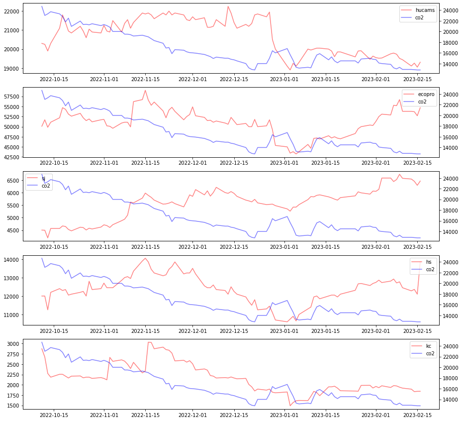
한국탄소배출권과 주가 그래프 그리기
fig = plt.figure(figsize=(15, 15))
ax1 = fig.add_subplot(5, 1, 1)
ax3 = fig.add_subplot(5, 1, 2)
ax5 = fig.add_subplot(5, 1, 3)
ax7 = fig.add_subplot(5, 1, 4)
ax9 = fig.add_subplot(5, 1, 5)
########################## 휴켐스
# y축 라벨 및 범위 지정
line1 = ax1.plot(df['date'], df['hucams_price'], color = 'red', alpha = 0.5, label='hucams')
ax1.tick_params(axis='y')
ax2 = ax1.twinx()
# y축 라벨 및 범위 지정
line2 = ax2.plot(df['date'], KAU22_df['종가'], color = 'blue', alpha = 0.5, label='co2')

lines = line1 + line2
labels = [l.get_label() for l in lines]
ax1.legend(lines, labels, loc='best')

########################### 에코프로
# y축 라벨 및 범위 지정
line1 = ax3.plot(df['date'], df['ecoprohn_price'], color = 'red', alpha = 0.5, label='ecopro')

ax4 = ax3.twinx()
# y축 라벨 및 범위 지정
line2 = ax4.plot(df['date'], KAU22_df['종가'], color = 'blue', alpha = 0.5, label='co2')

lines = line1 + line2
labels = [l.get_label() for l in lines]
ax3.legend(lines, labels, loc='upper right')

########################### 세종
# y축 라벨 및 범위 지정
line1 = ax5.plot(df['date'], df['sj_price'], color = 'red', alpha = 0.5, label='sj')

ax6 = ax5.twinx()
# y축 라벨 및 범위 지정
line2 = ax6.plot(df['date'], KAU22_df['종가'], color = 'blue', alpha = 0.5, label='co2')

lines = line1 + line2
labels = [l.get_label() for l in lines]
ax5.legend(lines, labels, loc='best')
############################# 휴성

line1 = ax7.plot(df['date'], df['hs_price'], color = 'red', alpha = 0.5, label='hs')
ax8 = ax7.twinx()
line2 = ax8.plot(df['date'], KAU22_df['종가'], color = 'blue', alpha = 0.5, label='co2')

lines = line1 + line2
labels = [l.get_label() for l in lines]
ax7.legend(lines, labels, loc='upper right')

############################ 코트렐

line1 = ax9.plot(df['date'], df['kc_price'], color = 'red', alpha = 0.5, label='kc')
ax10 = ax9.twinx()
line2 = ax10.plot(df['date'], KAU22_df['종가'], color = 'blue', alpha = 0.5, label='co2')

lines = line1 + line2
labels = [l.get_label() for l in lines]
ax9.legend(lines, labels, loc='best')

plt.show()
유럽 탄소배출권과 주가 관계
fig = plt.figure(figsize=(15, 15))
ax1 = fig.add_subplot(5, 1, 1)
ax3 = fig.add_subplot(5, 1, 2)
ax5 = fig.add_subplot(5, 1, 3)
ax7 = fig.add_subplot(5, 1, 4)
ax9 = fig.add_subplot(5, 1, 5)
########################## 휴켐스
# y축 라벨 및 범위 지정
line1 = ax1.plot(df['date'], df['hucams_price'], color = 'red', alpha = 0.5, label='hucams')
ax1.tick_params(axis='y')
ax2 = ax1.twinx()
# y축 라벨 및 범위 지정
line2 = ax2.plot(df['date'], eu_df['종가'], color = 'blue', alpha = 0.5, label='co2')

lines = line1 + line2
labels = [l.get_label() for l in lines]
ax1.legend(lines, labels, loc='best')

########################### 에코프로
# y축 라벨 및 범위 지정
line1 = ax3.plot(df['date'], df['ecoprohn_price'], color = 'red', alpha = 0.5, label='ecopro')

ax4 = ax3.twinx()
# y축 라벨 및 범위 지정
line2 = ax4.plot(df['date'], eu_df['종가'], color = 'blue', alpha = 0.5, label='co2')

lines = line1 + line2
labels = [l.get_label() for l in lines]
ax3.legend(lines, labels, loc='best')

########################### 세종
# y축 라벨 및 범위 지정
line1 = ax5.plot(df['date'], df['sj_price'], color = 'red', alpha = 0.5, label='sj')

ax6 = ax5.twinx()
# y축 라벨 및 범위 지정
line2 = ax6.plot(df['date'], eu_df['종가'], color = 'blue', alpha = 0.5, label='co2')

lines = line1 + line2
labels = [l.get_label() for l in lines]
ax5.legend(lines, labels, loc='best')
############################# 휴성

line1 = ax7.plot(df['date'], df['hs_price'], color = 'red', alpha = 0.5, label='hs')
ax8 = ax7.twinx()
line2 = ax8.plot(df['date'], eu_df['종가'], color = 'blue', alpha = 0.5, label='co2')

lines = line1 + line2
labels = [l.get_label() for l in lines]
ax7.legend(lines, labels, loc='best')

############################ 코트렐

line1 = ax9.plot(df['date'], df['kc_price'], color = 'red', alpha = 0.5, label='hs')
ax10 = ax9.twinx()
line2 = ax10.plot(df['date'], eu_df['종가'], color = 'blue', alpha = 0.5, label='co2')

lines = line1 + line2
labels = [l.get_label() for l in lines]
ax9.legend(lines, labels, loc='best')

plt.show()
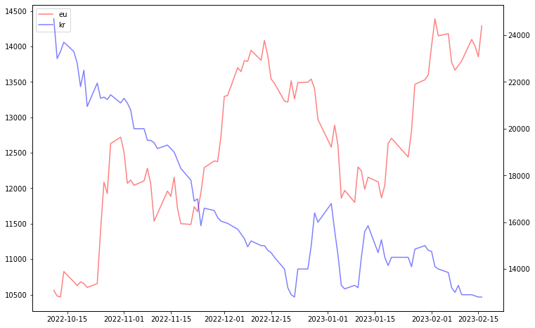
한국과 유럽의 탄소배출권 관계
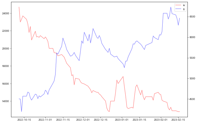
fig, ax1 = plt.subplots(figsize=(12, 8))
line1 = ax1.plot(df['date'], eu_df['종가'], color = 'red', alpha = 0.5, label='eu')
ax2 = ax1.twinx()
line2 = ax2.plot(df['date'], KAU22_df['종가'], color = 'blue', alpha = 0.5, label='kr')

lines = line1 + line2
labels = [l.get_label() for l in lines]
ax1.legend(lines, labels, loc='best')
plt.show()
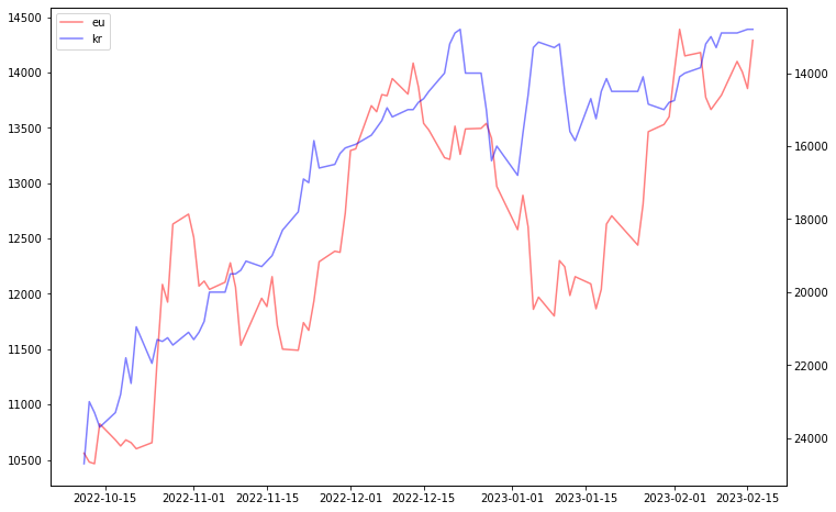
y축 반전
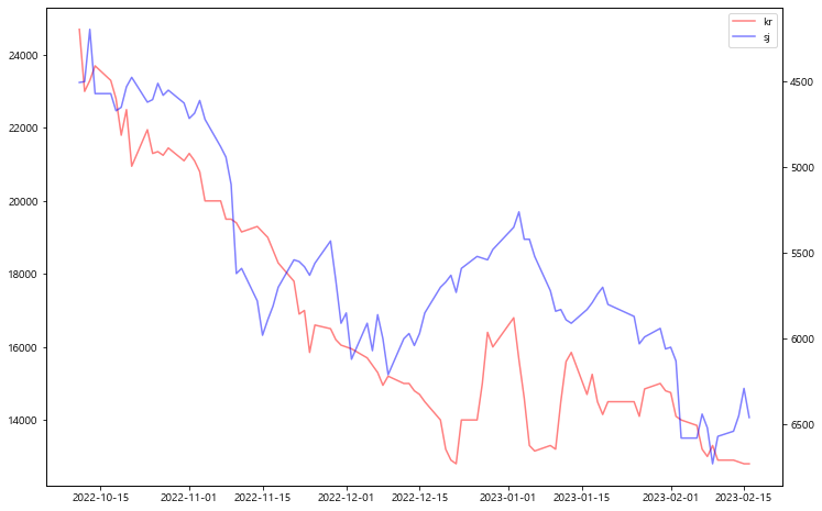
fig, ax1 = plt.subplots(figsize=(12, 8))
line1 = ax1.plot(df['date'], eu_df['종가'], color = 'red', alpha = 0.5, label='eu')
ax2 = ax1.twinx()
line2 = ax2.plot(df['date'], KAU22_df['종가'], color = 'blue', alpha = 0.5, label='kr')
lines = line1 + line2
labels = [l.get_label() for l in lines]
ax1.legend(lines, labels, loc='best')
plt.gca().invert_yaxis()
plt.show()
상관계수 히트맵
df01 = pd.DataFrame(data=df[['hucams_price','ecoprohn_price','hs_price','sj_price', 'kc_price']])
df01 = df01.set_axis([np.arange(0,90)], axis='index')
df02 = KAU22_df['종가']
df02 = df02.set_axis([np.arange(0,90)], axis='index')
df02 = pd.DataFrame(data = df02)
df03 = eu_df['종가']
df03 = df03.set_axis([np.arange(0,90)], axis='index')
df03 = pd.concat([df01,df02,df03], axis=1)
df03.columns = ['hucams_price','ecoprohn_price','hs_price','sj_price','kc_price','k_co2', 'eu_co2']

sns.set(style="white")
cor = df03.corr()
f, ax = plt.subplots(figsize=(12, 12))
sns.heatmap(cor, annot=True)
plt.title('co2 stock data correlation', size=30)
ax.set_xticklabels(list(df03.columns), size=15, rotation=90)
ax.set_yticklabels(list(df03.columns), size=15, rotation=0);
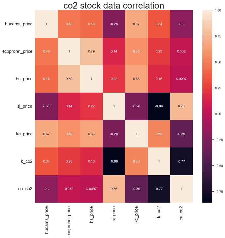
상관계수가 높은 관계 분석
한국과 주가 그래프
fig, ax1 = plt.subplots(figsize=(12, 8))
line1 = ax1.plot(df['date'], KAU22_df['종가'], color = 'red', alpha = 0.5, label='eu')
ax2 = ax1.twinx()
line2 = ax2.plot(df['date'], df['sj_price'], color = 'blue', alpha = 0.5, label='kr')

lines = line1 + line2
labels = [l.get_label() for l in lines]
ax1.legend(lines, labels, loc='best')
plt.show()
fig, ax1 = plt.subplots(figsize=(12, 8))
line1 = ax1.plot(df['date'], KAU22_df['종가'], color = 'red', alpha = 0.5, label='eu')
ax2 = ax1.twinx()
line2 = ax2.plot(df['date'], df['sj_price'], color = 'blue', alpha = 0.5, label='kr')

lines = line1 + line2
labels = [l.get_label() for l in lines]
ax1.legend(lines, labels, loc='best')
plt.gca().invert_yaxis()
plt.show()
유럽과 주가 그래프
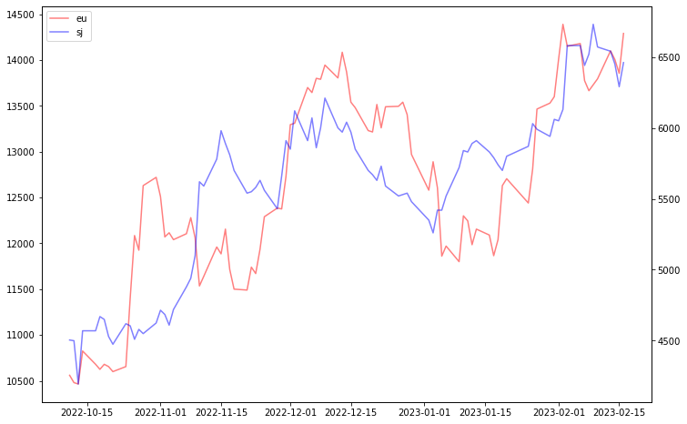
fig, ax1 = plt.subplots(figsize=(12, 8))
line1 = ax1.plot(df['date'], eu_df['종가'], color = 'red', alpha = 0.5, label='eu')
ax2 = ax1.twinx()
line2 = ax2.plot(df['date'], df['sj_price'], color = 'blue', alpha = 0.5, label='sj')
lines = line1 + line2
labels = [l.get_label() for l in lines]
ax1.legend(lines, labels, loc='best')
plt.show()
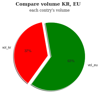
유럽 배출권과 한국 배출권 거래량 비교
eu_df['거래량'] = eu_df['거래량'].str.replace(',', '')
eu_df['거래량'] = eu_df['거래량'].astype('int')
KAU22_df['거래량'] = KAU22_df['거래량'].str.replace(',', '')
KAU22_df['거래량'] = KAU22_df['거래량'].astype('int')
vol_kr = KAU22_df['거래량'].mean()
vol_eu = eu_df['거래량'].mean()
ratio = [vol_kr, vol_eu]
eu_df['거래량'] = eu_df['거래량'].str.replace(',', '')
eu_df['거래량'] = eu_df['거래량'].astype('int')
KAU22_df['거래량'] = KAU22_df['거래량'].str.replace(',', '')
KAU22_df['거래량'] = KAU22_df['거래량'].astype('int')
vol_kr = KAU22_df['거래량'].mean()
vol_eu = eu_df['거래량'].mean()
ratio = [vol_kr, vol_eu]
plt.figure(figsize=(5, 5))
plt.pie(ratio, labels=['vol_kr', 'vol_eu'], autopct='%0.f%%', startangle=100,
        explode=[0.05, 0.05], shadow=True, colors=['red', 'green'])
plt.suptitle('Compare KR volume with EU volume', fontfamily='serif', fontsize=15, fontweight='bold')
plt.title('each contry\'s volume', fontfamily='serif', fontsize=12)
plt.show()
분석
1. 한국 탄소 배출권 가격과 관련주 분석
A. 그래프 분석
- 기간 : 2022년 10월 1일 ~ 2023년 3월 1일 / 약 5개월
- 분석 내용
- 탄소 배출권 관련주로 소개되어지는 종목들 중 탄소 배출권 가격과 관련이 있어보이는 종목은 코트렐로 탄소배출권 가격보다 조금 앞서서 변동하는 추세 보인다.
- 탄소 배출권 가격과 코트렐은 유사하게 우하향하는 그래프를 보인다.
- 나머지 종목들은 우상향하는 지표를 보여준다
B. 예측 및 대응
- 2023년 이후 코트렐의 주가에 따라 탄소 배출권 가격이 움직이는 것을 보아 코트렐의 주가 변동을 보고 탄소 배출권의 가격을 예측할 수 있지 않을까 싶다.
- 한국의 탄소배출권 가격이 우하향하는 이유는 ‘이월 제한’ 제도로 보인다. 기업들의 배출권 사재기를 막기 위해 올해 쓰고남은 배출권 가운데 다음 해로 이월하는 물량을 규제하는 것이다. 내년부터 이월하는 물량을 1배로 정하지만 올해에는 매도량의 2배로 많기 때문이다.
(출처 : https://www.hani.co.kr/arti/economy/economy_general/1100658.html)
2. 유럽 탄소 배출권과 한국 탄소 배출권 관계
A. 그래프 분석
- 그래프 설명
- 유럽의 탄소 배출권은 우상향하는 그래프
- 한국의 탄소 배출권은 우하향하는 그래프
- 기간 : 2022년 10월 1일 ~ 2023년 3월 1일 / 약 5개월
- 분석내용
- 유럽의 탄소배출권과 한국의 탄소배출권의 가격 변동은 정반대이다.
- 한국의 '이월 제한'제도로 인해 가격이 계속 감소한다.
B. 예측
- 이월 제한이 매도량의 2배로 많아지는 올해에는 계속 우리나라 탄소배출권 가격이 감소할것 같다.
- 내년에는 우리나라 탄소배출권 이월 제한이 1배로 내려감에 따라 가격이 증가할 수 있을것 같다.
- 유럽의 경우 탄소배출권에 관심이 많아 가격이 계속 우상향할 것 같다.

가보자가보자~