Sigmoid & TanH

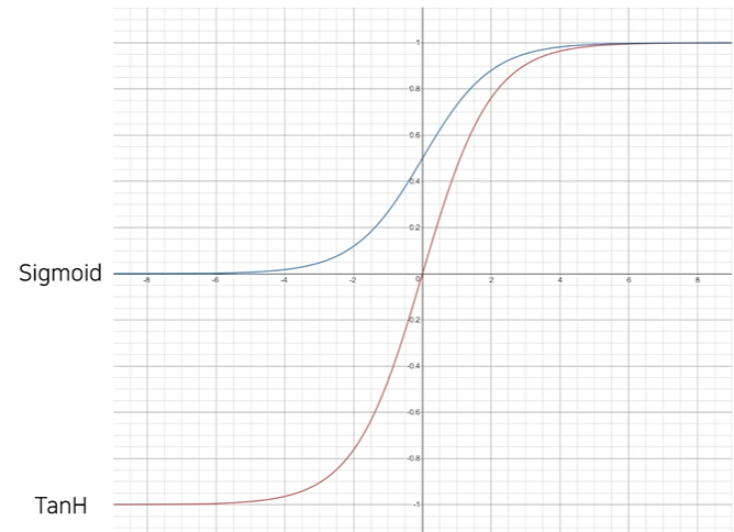
Sigmoid

import torch
import torch.nn as nn
from matplotlib import pyplot as plt

# 정규분포 생성
x = torch.sort(torch.randn(100) * 10)[0] # 10을 곱해서 값을 크게 만듬

act = nn.Sigmoid()
print(act(x)) # 0~1사이의 값이 나옴
print(torch.sigmoid(x))
plt.plot(x.numpy(), torch.sigmoid(x).numpy())
plt.show()

TanH

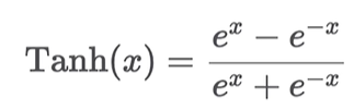
act = nn.Tanh()
print(act(x)) # -1 ~ 1 사이의 값이 나옴
print(torch.tang(x)) 
plt.plot(x.numpy(), torch.tanh(x).numpy())
plt.show()

Logistic Regression

• 이름은 Regression이지만 사실은 이진 분류(binar classification) 문제
  • Regression
    • Target value : real-value vector
  • Classification
    • Traget value : categorical value
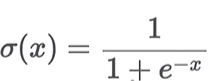
• 기존의 선형회귀(Linear Regression)과 달리, Linear Layer의 결과물에 sigmoid함수를 활용하여 출력값 y'를 계산
  • sigmoid의 출력 값은 0에서 1이므로, 확률 값 p(y|x)으로 생각해볼 수 있다.
• Regression의 경우에는 보통 손실함수 MSELoss를 활용하여 파라미터를 최적화
• Classification의 경우에는 BCELoss를 활용하여 파라미터를 최적화하며, Accuracy를 통해 우리는 모델의 성능을 평가할 수 있다.
  • BCELoss의 경우에는 확률/통계, 정보 이론과 밀접한 관련이 있다.

structure

• Linear Regression과 비슷한 구조이나, 마지막에 Sigmoid 함수를 통과시킴
• Sigmoid 함수를 사용하기 때문에 1(True)과 0(False) 사이의 값을 반환
  • 각 항목에 대하여 0.5 이상이면 True
  • 각 항목에 대하여 0.5 이하이면 False
• 출력 벡터의 각 차원별로 하나의 문제

Binary Classification

• sigmoid의 출력 값은 0에서 1
• 따라서 확률 값 p(y|X)으로 생각해볼 수 있음
• 실제 정답이 1이라면, 모델은 확률 값이 최대한 커지도록 학습될 것

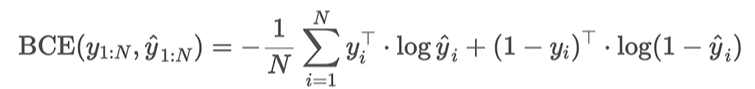
Binary Cross Entropy (BCE) Loss Function

• N개의 vector들이 주어졌을 때의 수식
• yi의 값에 따라 수식의 왼쪽 term과 오른쪽 term이 on/off

실습

EDA

import pandas as pd
import seaborn as sns
import matplotlib.pyplot as plt
# sklearn에 있는 데이터셋 사용
from sklearn.datasets import load_breast_cancer
cancer = load_breast_cancer()

# 데이터프레임으로 변경
df = pd.DataFrame(cancer.data, columns=cancer.feature_names)
# targetvalue 컬럼을 추가
df['class'] = cancer.target

# Pair plot with mean features
sns.pairplot(df[['class'] + list(df.columns[:10])])
plt.show

# Pair plot with std features
sns.pairplot(df[['class'] + list(df.columns[10:20])])
plt.show

# Pair plot with worst features
sns.pairplot(df[['class'] + list(df.columns[20:30])])
plt.show

cols = ['mean radius', 'mean texture', 'mean smoothness', 'mean compactness',
		' mean concave points', 'worst radius', 'worst texture', 'worst smoothness', 'worst compactness', 'worst concave points', 'class']
for c in cols[:-1]:
	sns.histplot(df, x=c, hue=cols[-1], bins=50, stat='probability')
    plt.show()

Train Model with PyTorch

import torch
import torch.nn as nn
import torch.nn.functional as F
import torch.optim as optim
data = torch.from_numpy(df[cols].values).float()

# x와 y를 split
x = data[:, :-1]
y = data[:, -1:]

# 학습을 위한 설정
n_epochs = 200000
learning_rate = 1e-2
print_interval = 10000

# 모델 정의
class MyModel(nn.Module):

    def __init__(self, input_dim, output_dim):
    	self.input_dim = input_dim
        self.output_dim = output_dim

        super().__init__()

        self.linear = nn.Linear(input_dim, output_dim)
        self.act = nn.Sigmoid()

def forward(self, x):
	# |x| = (batch_size, input_dim)
    y = self.act(self.linear(x)) # (n,1)
    # |y| = (batch_size, output_dim)
    return y

모델 선언

model = MyModel(input_dim = x.size(-1),
output_dim = y.size(-1))
crit = nn.BCELoss()
optimizer = optim.SGD(model.parameters(),
lr = learning_rate)

모델 실행

for i in range(n_epochs):
y_hay = model(x) # 사이즈는 y랑 동일(n,1)
loss = crit(y_hay, y) # 둘이 연산해서 BSELoss 계산

optimizer.zero_grad() # gradient 초기화
loss.backward() # loss에 대해 미분

optimizer.step()

if (i+1) % print_interval == 0:
	print("Epoch %d: loss = %.4e' % (i + 1, loss)

결과 확인

correct_cnt = (y ==(y_hat > .5)).sum() # 맞은 갯수 출력
total_cnt = float(y.size(0)) # 총사이즈

print('Accuracy: %.4f' % (correct_cnt / total_cnt))

df = pd.DataFrame(torch.cat([y, y_hat], dim=1).detach().numpy(),
					columns=['y', 'y_hat'])

sns.histplot(df, x='y_hat', hue='y', bins=50, stat='probability')
plt.show()