머신러닝-5단계(클래스(target) 불균형, y_test 값 x)

0. 클래스 불균형

• 실제 작업에서는 target 데이터가 불균형있게 나타나 있는 경우가 많다.
  • ex) 공장 장비 고장을 예측하고 싶은 경우, 당연히 정상작동의 경우 980건 비정상작동의 경우 15건 이렇게 불균형인 경우.

---

• 불균형인 상태에서 y_pred를 구하고 값을 비교해보면 accuracy가 높지만 target의 납은 값에 대한 recall은 현저히 낮다.
• 해결 방법으로는 1) Under Sampling 2) Over Sampling이 있다.

---

• Under/Over sampling은 확률로 나타내는 정규화와 비슷하지만, 정규화와 다른 점이 있다.
  • fit을 x_train과 y_train 2개에 진행한다.
  • x_test는 건드리지 않는다.

1. 불균형 상태에서 그냥 진행

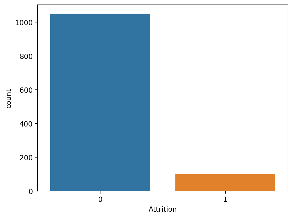
# Target 확인
print(data['Attrition'].value_counts())
sns.countplot(x='Attrition', data=data)
<출력>
0    1050
1     100

# 선언하기
model = RandomForestClassifier(max_depth=5, random_state=1)

# 학습하기
model.fit(x_train, y_train)

# 예측하기
y_pred = model.predict(x_test)

# 평가하기
print(confusion_matrix(y_test, y_pred))
print(classification_report(y_test, y_pred))
<출력>
[[317   1]
 [ 26   1]]
              precision    recall  f1-score   support

           0       0.92      1.00      0.96       318
           1       0.50      0.04      0.07        27

    accuracy                           0.92       345
   macro avg       0.71      0.52      0.51       345
weighted avg       0.89      0.92      0.89       345

---

2. Under Sampling

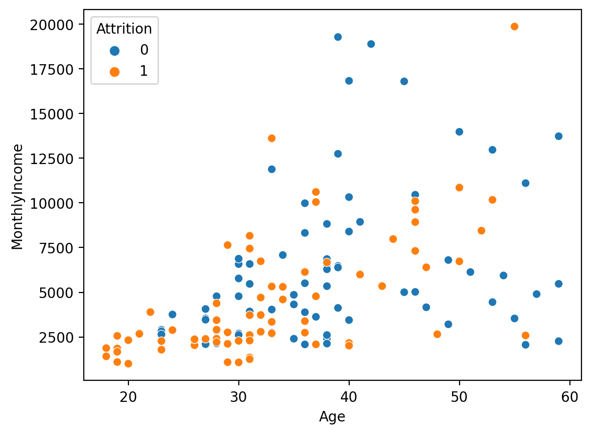
# 불러오기
from imblearn.under_sampling import RandomUnderSampler

# under sampling
under_sample = RandomUnderSampler()
u_x_train, u_y_train = under_sample.fit_resample(x_train, y_train)

# 확인
print('전:', np.bincount(y_train))
print('후:', np.bincount(u_y_train))
<출력>
전: [732  73]
후: [73 73]

# 학습 데이터 분포 확인
sns.scatterplot(x='Age', y='MonthlyIncome', hue=u_y_train, data=u_x_train)
<출력>

# 모델 성능 확인

# 선언하기
model = RandomForestClassifier(max_depth=5, random_state=1)

# 학습하기
model.fit(u_x_train, u_y_train)

# 예측하기
y_pred = model.predict(x_test)

# 평가하기
print(confusion_matrix(y_test, y_pred))
print(classification_report(y_test, y_pred))
<출력>
[[254  64]
 [ 12  15]]
              precision    recall  f1-score   support

           0       0.95      0.80      0.87       318
           1       0.19      0.56      0.28        27

    accuracy                           0.78       345
   macro avg       0.57      0.68      0.58       345
weighted avg       0.90      0.78      0.82       345

---

3. over sampling

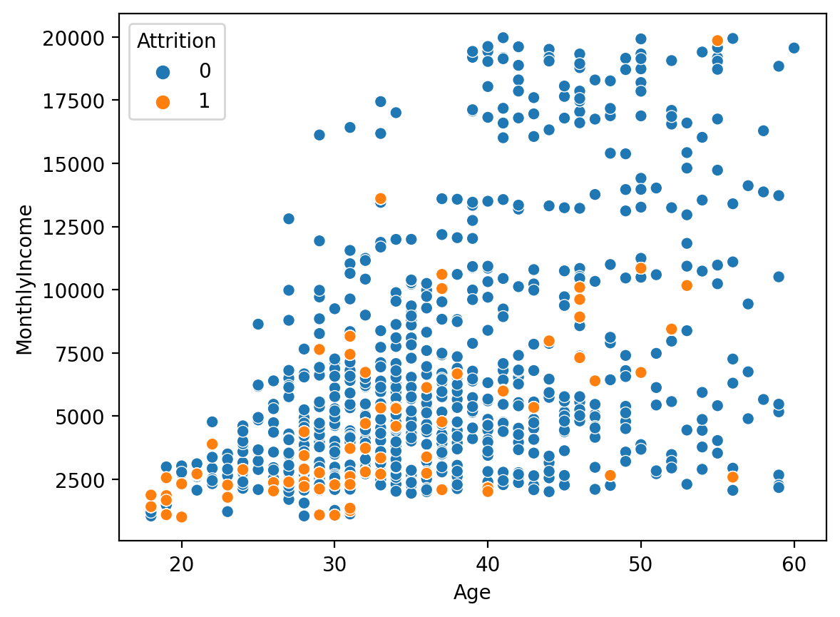
# 불러오기
from imblearn.over_sampling import RandomOverSampler

# Over Sampling
over_sample = RandomOverSampler()
o_x_train, o_y_train = over_sample.fit_resample(x_train, y_train)

# 확인
print('전:', np.bincount(y_train))
print('후:', np.bincount(o_y_train))
<출력>
전: [732  73]
후: [732 732]

# 학습 데이터 분포 확인
sns.scatterplot(x='Age', y='MonthlyIncome', hue=o_y_train, data=o_x_train)
<출력>

#모델 성능 확인
print(confusion_matrix(y_test, y_pred))
print(classification_report(y_test, y_pred))
[[283  35]
 [ 16  11]]
              precision    recall  f1-score   support

           0       0.95      0.89      0.92       318
           1       0.24      0.41      0.30        27

    accuracy                           0.85       345
   macro avg       0.59      0.65      0.61       345
weighted avg       0.89      0.85      0.87       345

---

4. over sampling #2

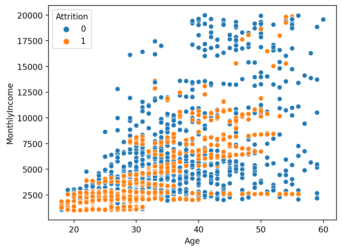
• SMOTE를 사용하는 방법이며, 가장 많이 사용하는 oversampling 기법이다.

# 불러오기
from imblearn.over_sampling import SMOTE

# Over Sampling
smote = SMOTE()
s_x_train, s_y_train = smote.fit_resample(x_train, y_train)

# 확인
print('전:', np.bincount(y_train))
print('후:', np.bincount(s_y_train))

# 학습 데이터 분포 확인
sns.scatterplot(x='Age', y='MonthlyIncome', hue=s_y_train, data=s_x_train)
<출력>

# 평가하기
print(confusion_matrix(y_test, y_pred))
print(classification_report(y_test, y_pred))
<출력>
[[296  22]
 [ 17  10]]
              precision    recall  f1-score   support

           0       0.95      0.93      0.94       318
           1       0.31      0.37      0.34        27

    accuracy                           0.89       345
   macro avg       0.63      0.65      0.64       345
weighted avg       0.90      0.89      0.89       345

---